
Network as a Service (NaaS) PlayBook
1. Tx Network High-Level Design Introduction
The Tx Network High-Level Design (HLD) module provides the NaaS operator with background information and methodologies to elaborate a HLD for a Tx network. It provides guidelines about how to design the transport network that interconnects disparate networks, including a radio access network (RAN) and data centers. It further provides instruction about how to transform guidelines into actual design parameters that is necessary for Tx network HLD development.
The main output of this module is the Tx network HLD that includes, among others, the transport design that specifies physical and logical topology, the transport solution to be implemented, and a high-level bill of quantities (BOQ). The business case can be analyzed with this information. This module will guide the NaaS operator through the process of generating a technically compliant HLD to speed decision-making and the related deployment process.
1.1 Module Objectives
This module will enable a NaaS operator to standup, run, and manage a Tx network HLD initiative. The specific objectives of this module are to:
- Provide an information base and fundamentals to perform tasks associated with Tx network HLD.
- Provide detailed how-to instruction regarding key HLD engineering tasks.
- Provide an overview of the end-to-end Tx network HLD process, with instructions for tailoring it to specific NaaS environments.
- Provide guidelines to develop a formal Tx network HLD recommendation.
1.2 Module Framework
The module framework in Figure 1 describes the structure, interactions, and dependencies among NaaS operator areas.
Strategic plan and scope, along with high-level network architecture drive the strategic decisions to forthcoming phases. Network design is the first step in an implementation strategy supported by supply chain management.
The Tx network HLD module is included within the network design area and has direct relation with RAN HLD and mobile core HLD. The generated output of this module will serve as a required input for the Tx network LLD module.
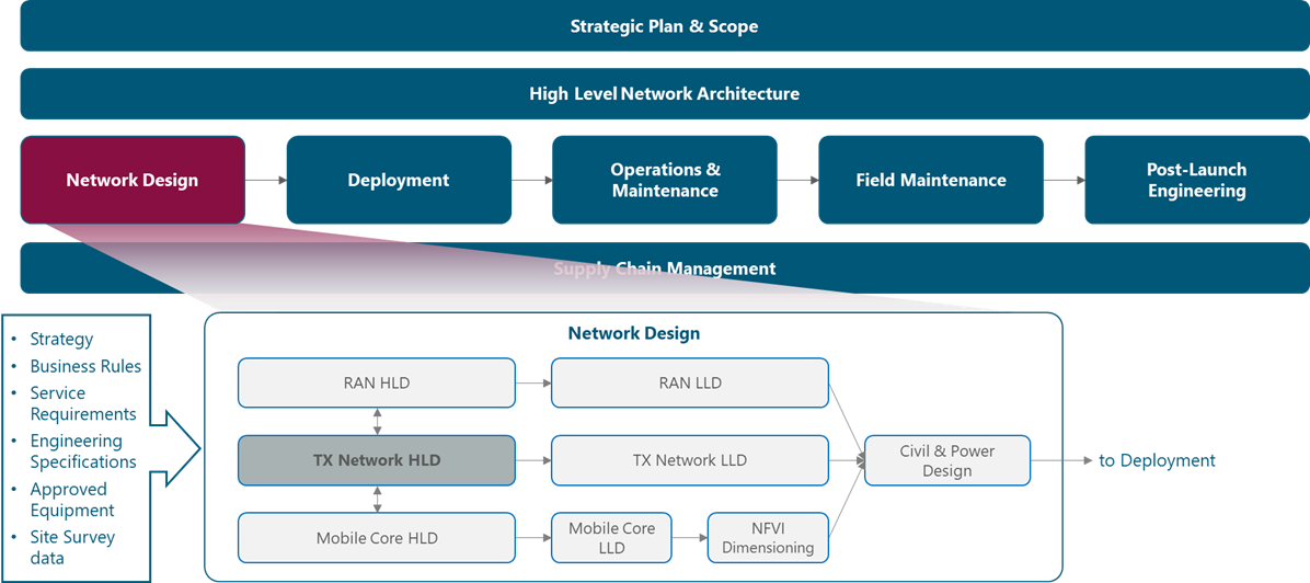
Figure 1 ‒ Module framework
Figure 2 presents the Tx network HLD functional view, where the main functional components are exhibited. Critical module inputs are further described and examined in Section 2.2. In addition, guidance and methodologies to execute the tasks included within each function are described in Section 3.
Figure 2 ‒ Module functional view
The remainder of this module is structured as follows: Section 2 is a high-level overview of the Tx network fundamentals involved in its design. Once such knowledge is acquired, Section 3 focuses on showing a hands-on view of the involved design tasks. Section 4 organizes the tasks on an end-to-end process flow that can be used as-is, or be adapted by NaaS operators to match their particular conditions. To conclude, Section 5 illustrates how to integrate previous elements in a comprehensive HLD recommendation.
Review of fundamental transport technologies are found in the Learning Repository and is a useful prerequisite to this module.
2 HLD Fundamentals
General overview of the baseline concepts to develop a Tx network design.
2.1 Tx Network Environment
In a mobile environment, the transport network interconnects disparate networks, including the RAN, data centers, and external networks. Figure 3 displays the architecture of a typical transport network.
Figure 3 ‒ Typical transport network
Mobile networks are ubiquitous and support a mix of traffic types originating from and terminating to mobile devices. All of this traffic must be conveyed between the mobile cellular base stations and transport network. For this reason, a number of aggregation levels exist on the transport network that for most NaaS operators can be classified as either: last-mile or aggregation level.
The implementation of 4G long-term evolution (LTE) imposes some requirements on transport networks, such as more network capacity and latency reduction. These are better served through terrestrial technologies (fiber optic and microwave). But in rural areas this becomes a challenge because satellite transport is usually the only feasible technology. For this reason, transport network infrastructure is an essential component of the NaaS operator network; its design must be performed with optimal processes and techniques.
2.1.1 Requirements for Transport Network
Capacity: Compared to 2G and 3G, LTE base stations support a considerable amount of traffic. In addition to user traffic, control, management, and synchronization traffic must be considered. A detailed explanation regarding traffic models is provided in Section 3.4.
Latency: In addition to capacity increase, latency reduction is one of the key goals of LTE deployments. The delay requirements for the transport depend on the end-to-end delay of end customer applications and on the delay budget given to the transport. Latency requirements can be an important limitation for some transport technologies such as satellite and can directly affect its feasibility.
Availability: The availability requirements of the transport network are derived from the those of the end-user service. A typical requirement for a transport network in a rural environment could be an availability value of 99.95%. In most cases availability is dominated by the last-mile link.
2.2 Network Design Inputs Description
This section analyzes the module input data and their respective candidate sources, as presented in Table 1. In addition, the impact of module inputs on the design process is examined.
|
Input Required |
Description |
Candidate Source |
Impact |
|
RAN HLD Design |
Describes parameters related with RAN solution (site location, RAN equipment, covered population) |
RAN HLD Module |
– The total number of RAN sites determines tool selection to perform the transport feasibility analysis (details in following sections) |
|
Tx & IP Architecture |
Includes the technologies, equipment, and protocols to be considered in the design |
Tx & IP Architecture Module |
– Establishes the available transport technologies to be evaluated during the feasibility analysis and their respective technical considerations |
|
Operator |
Consists on consolidated information regarding operating data network (e.g., existing network elements, implemented protocols) |
– Network operators tools (e.g., inventory, OSSs) |
– Contains the existing transport nodes and technologies to be considered during feasibility analysis |
|
Offered Service Catalogue |
Contains a list of services to be provided and is an output from Tx & IP Architecture Module |
Tx & IP Architecture Module |
– Offered services determine the service level requirements for the transport network |
|
Commercial Criteria |
Guideline criteria to follow during design process |
Commercial area |
– Establishes guidelines to prioritize use of one transport provider over others during the feasibility analysis – Establishes the budget to acquire design tools during feasibility analysis |
Table 1 ‒ Module inputs analysis
2.3 Transport Solution Feasibility Analysis
This section describes the feasibility considerations for different transport technologies to be used on the transport network. When it comes to technical transport solutions, mobile operators have several at their disposal. Mobile operators prefer fiber optic where available ‒ especially in city centers ‒ but microwave is the mainstay for last-mile traffic. Satellite transport is mainly deployed where existing transport infrastructure isn’t available.
2.3.1 Fiber Optic Technology
Fiber optic is the mainstay wired transport in mobile operator networks when its available because of its significant, inherent bandwidth-carrying ability. Several other techniques can be used to offset any bandwidth constraints and essentially render fiber assets future-proof.
While fiber optic has tremendous operational capacity, its main limitation is its cost and deployment logistics. Moreover, it can take several months to provision each cell site with fiber optic transport.
The fundamental aspects of fiber optic technology design are discussed in the Primer on Fiber Optic Technologies Principles.
2.3.2 Microwave Technology
Most operators heavily rely on microwave transport solutions in the 5 GHz – 80 GHz bands (in rural environments, frequencies above 15GHz are not generally feasible). Microwave is a low-cost option for mobile transport, as it can be deployed in a matter of days and support a range of up to several tens of kilometers.
The main limitation of microwave links is its line of sight (LOS) requirement between transmitter and receiver. This represents a drawback for its implementation, especially in rural areas due to steep terrain conditions that often exist. In addition, in many cases microwave requires a license to be obtained. And in high frequencies, microwave links are subject to atmospheric effects or rain fade, which can attenuate the signal and limit its range.
The fundamental aspects of microwave technology design are discussed in the Primer on Microwave Technologies Principles..
2.3.3 Satellite Technology
Satellite technology is deployed in fringe network areas, usually in rural locations within emerging markets. It may be deployed as a temporary measure as an operator waits for regulatory microwave licenses to be approved. Coverage is determined by satellite footprint. More details are provided in Section 3.
Table 2 presents a comparison of satellite orbits.
|
Orbit |
GEO |
MEO |
LEO |
|
Distance |
35,800 km |
2,000km-35,000km |
160km-2,000km |
|
Latency |
250-500 ms |
60-250 ms |
30-50 ms |
|
Throughput |
Up to 500 Mbps |
Up to 800 Mbps |
1Gbps+ *(See NOTE) |
|
No HO |
2-3 hours |
15-20 min |
Table 2 ‒ Satellite orbit comparison
*NOTE: As LEO systems have not been commercially launched, the 1Gbps value is used as a theoretical reference.
The cost of satellite terminal equipment located at the base station is in line with microwave equipment. However, the OPEX burden generated by the satellite service fee can impact the business case.
The fundamental aspects of satellite technology design are discussed in the Primer on Satellite Technologies Principles.
2.4 Physical Topology Design
As stated in Section 2.1, a typical transport network consists of two domains: Last-mile and aggregation. In most cases there might exist a connection provided by a third party network to connect to core elements. Domain borders are mostly defined by the technology and topology used within the domain. Domain characteristics in terms of physical topology are:
Figure 4 displays the transport network structure:
Figure 4 ‒ Basic structure of a mobile transport network
The depicted structure considers various physical technologies and topologies. From left to right, the last-mile connects a demarcation device (usually deployed at the cell site) to a first stage of traffic grooming and concentration. In turn, the aggregation network further aggregates traffic, adapts any technology change, and provides the hand over point to a higher level of aggregation network.
Physical connectivity represents any technology that can be used to connect nodes (details in section 3). In addition, a networking layer is implemented on top of the physical layer; it embraces all possible logical architectures needed to steer LTE traffic and applications. Details on network topology design are covered in the Tx LLD Module.
2.5 Capacity Planning Process
In simple terms, the transport network should be dimensioned to provide reliable service to users. They should be able to connect to the network and use subscribed services anytime inside the coverage area ‒ where service outages or connectivity problems should be rare. To achieve this, a capacity planning analysis must be performed to determine the traffic the transport network must support.
2.6 Transport Solution Definition
An assessment of implementing a transport network or link is dependent on feasible transport solutions and capacity requirements, as well as the following implications.
Feasible Transport Solutions Feasibility analysis is an essential step in defining the transport solution to be deployed, for not all the solutions are appropriate in rural areas. Thus, feasibility might be the most important constraint in selecting a transport technology.
Capacity Requirements In wireless-based solutions (MW and satellite), it’s essential to validate that sufficient capacity exists to satisfy traffic requirements. Capacity planning assesses how much traffic can be supported by transport technologies.
Deployment Cost Deployment cost can be a essential criterion when a network operator is faced with deploying several cell sites in one year.
Time to Deploy and Licensing Network operators are often under pressure to get a cell site operational as quickly as possible. Having to wait several months for a fiber optic connection to be provisioned to a cell site can prevent its selection in the near term.
Table 3 presents a high-level comparison of technology parameters to be implemented on the transport network.
|
Parameter |
Fiber Optic |
Microwave |
Satellite |
|
Future-proof Available Bandwidth |
High |
Medium |
Low |
|
Deployment Cost |
High |
Low |
Medium |
|
Interference Immunity |
Very-high |
Medium |
Medium |
|
Range (km) |
<80 |
<30* (5-15GHz) |
Subject to satellite footprint |
|
Time to Deploy |
Months |
Weeks |
Weeks |
|
Licensed Required |
No |
Both (Licensed/Unlicensed) |
No |
Table 3 ‒ Transport technologies high-level comparison
*Note: Typical value; however, microwave links can be engineered to reach larger distances.
3 Functions & Methodologies
This section presents recommended methodologies to perform critical tasks/subtasks involved in the Tx network design process.
3.1 Fiber Optic Path Design
3.1.1 Right of Way Definition
An actual fiber route will be determined by the physical locations along the way, local building codes or laws, and other considerations involved in the design. Laying fiber optic cable may cross long lengths of open fields; run along paved rural or urban roads; cross roads, ravines, rivers, or lakes; or ‒ more likely ‒ some combination thereof. It could require buried, aerial, or underwater cables. Cable may be in conduit, innerduct, or direct-buried; aerial cables can be self-supporting or lashed to a messenger. In rural areas, aerial cable is the most common deployment due to its low cost and fast implementation.
For this reason, a NaaS operator must define a set of rules (i.e., rights of way) that specify criteria to follow during fiber optic laying design. This set of rules prioritize the previously mentioned characteristics according to the operators requirements.
3.1.2 Geospatial Database
A geospatial database must be consolidated by the operator during the design process. It should contain road information, topographical data, and sometimes satellite images overlaid on roads (when available).
Other kinds of data to be considered are existing conduit, property boundaries, easements, gas pipelines, and areas of special interest. Each provides extra information that can be used to generate a fiber laying designeither things to avoid (e.g., gas pipes) or ways to save cost (e.g., existing conduit).
Streets and addresses are available as open source data in many places in the world (e.g., OpenStreetMap), but the remainder usually has to be sourced from local government councils or companies. A key step in using geospatial data is to confirm its quality, structure, and format so it can be useful for design.
3.1.3 Fiber Path Design
An identification of multiple paths to link origin and destination must be performed in designing the fiber optic path. These alternatives will likely include a combination of multiple rights of ways and have various optical lengths.
Although the specific steps can vary depending on the selected GIS tool, general steps in performing fiber path design are:
- Load the locations of origin and destination nodes in a GIS tool.
- Identify available routes linking the origin and destination nodes. Draw the path using the options provided by the GIS tool. Figure 5 shows an example of multiple path alternatives (A, B, C) from origin to destination nodes.
Figure 5 ‒ Example of fiber path design
- Using the GIS tool options, measure lengths of the alternatives; these represent the optical length of each path. Typically 20% is added as a margin to each measurement. Figure 5 shows each path length, with option A being the longest.
- Rank the alternatives to prioritize those that better comply with defined rights of ways having minimum length. A higher-ranked alternative will be selected as the final route.
3.1.4 Fiber Path Reporting
Once the fiber route is designed, create a path design report that includes:
3.2 Microwave Line of Sight (LOS) Verification
A microwave LOS analysis determines whether a signal path is available between transmitting and receiving antennas. This assures that a clearance of the first Fresnel ellipsoid is achieved.
The absence of relevant obstacles along the path to ensure LOS clearance is based on geometrical calculations. These require topographical databases used for path profile extraction. Profiles are to be drawn in a path profile diagram, along with the expected path taken by a radio signal. The diagram will enable comparison of both plots (profile and radio signal path) to analyze possible diffraction or reflection effects of the terrain.
3.2.1 Digital Terrain Databases
In general, most propagation predictions are based on detailed topographical information. This information is provided by digital terrain elevation (DTE) models composed by digital terrain topographical databases and represented in the form of digital terrain maps. The models provide accurate information that can be used to evaluate path clearance and potential loss associated with diffraction. They’ll also be used in the algorithm required for determining interference to/from other stations of the link, or arriving to/from other radio systems sharing the same bands.
Depending on the tool selected to perform the design, DTE models are often included. If not, some DTEs are available as open source data in many places in the world (e.g., Google Maps Elevation API).
3.2.2 Profile Extraction, Clearance, and Obstructions
The LOS clearance analysis is based on studying terrain heights between stations of the hop and along the path profile; comparing these with the expected path followed by the radio signal (first Fresnel ellipsoid).
Although specific steps can vary depending on the selected verification tool, the general steps to perform microwave LOS verification are:
- Load the locations of the origin and destination nodes in the tool. Figure 6 displays the analysis for one site when two transport nodes are considered.
Figure 6 ‒ Example of microwave link design
- Load tower height information for each of the sites. As a margin, typically each height is considered to be 3m below actual to account for space to implement the MW antennas.
- Using options provided by the selected tool, measure the distance between the sites; this represents the microwave link length. Figure 6 shows two links, with option A having the longest length.
- Select the frequency to be used based on link length (11GHz in Figure 6).
- Generate the microwave link profile using options provided by the selected tool.
- Verify that the first Fresnel zone is obstacle free (LOS is validated when there are none). Figure 7 depicts profiles generated for the example, where LOS is only validated for link B.
Figure 7 ‒ LOS validation during microwave link design
3.2.3 Microwave LOS Validation Reporting
Once LOS clearance has been validated, create a link design report that includes the following information:
3.3 Satellite Link Validation
3.3.1 Satellite Coverage Verification
The satellite footprint ‒ the ground area covered by its radiation ‒ should be obtained to validate satellite coverage. Footprint size depends on satellite location within its orbit, the shape and size of beam produced, and its distance from Earth. Footprints usually show estimated signal strength in each area as measured in decibel watts (dBW).
The majority of commercial satellites provide their footprint in respective documentation, or you can access it from satellite footprint databases (e.g., Satbeams at satbeams.com/footprints).
To establish a satellite link according to service level requirements, the minimum signal strength on reception must be defined based on satellite service provider specifications. Given this data, coverage validation for a specific site location can be performed using GIS operations. The aim is to determine whether the location is inside the polygon defined by the footprint and has the minimum level of strength required for the implementation. Depending on the selected tool using methodology in section 4, these operations can be processed in batch mode.
3.3.2 Satellite Parameter Calculation
The methodology presented in this section helps determine parameters for geostationary satellites. Azimuth and elevation angles are referred to as the look angles from the earth station (EA) to the satellite. Figure 8 shows the geometry and definitions of look angles with respect to the earth station reference.
Figure 8 ‒ Look angles with respect to ES reference
The azimuth angle, ϕ, is measured from true north in an eastward direction to the projection of the satellite path onto the local horizontal plane. The elevation angle, θ, is the angular distance between the satellite and the observers local horizon or the observers local vertical plane.
Look angles from an earth station to a satellite are determined from:
![]()
![]()
Where:
S = Satellite longitude in degrees
N = Site longitude in degrees
L = Site latitude in degrees
![]()
3.3.3 Satellite Coverage Validation Reporting
Once satellite coverage is validated and look angles calculated, create a link design report that includes the following information:
3.4 Capacity Forecast Analysis
This section presents a methodology to obtain the total amount of traffic the transport network needs to support. It can be summarized as:
3.4.1 Sector Throughput
In a typical LTE cell, throughput varies due to the averaging effect of much user equipment (UEs) using the network. It’s during quiet times that peak (and thus last-mile link) throughputs occur, when one UE with a good link has the entire cell to itself. Last-mile provisioning should ensure that advertised peak rates are at least feasible. Figure 9 shows sector throughput variations.
Figure 9 ‒ Illustration of cell throughput variations
Define the following inputs to model traffic behavior presented in Figure 9:
 ‒ average capacity used by eNodeB, calculated by Eq. 1)
 ‒ the relation between peak and average capacity. For an LTE downlink, peak is around 4 ‒ 6 times average throughput
 -
 ‒ required peak capacity, calculated by multiplying average capacity by the peak-to-average-ratio
 - ‒ is a parameter an operator can obtain from the existing network or previous deployment. If not available, the typical values of an LTE system can be considered. Table 4 displays cell average throughput for various scenarios and bandwidths.
|
Bandwidth |
Scenario |
Sector Average Throughput |
|
|
DL (Mbps) |
UL (Mbps) |
||
|
5 |
Urban |
8 |
5 |
|
Suburban |
6 |
3 |
|
|
10 |
Urban |
17 |
10 |
|
Suburban |
13 |
7 |
|
|
15 |
Urban |
25 |
15 |
|
Suburban |
20 |
10 |
|
|
20 |
Urban |
33 |
20 |
|
Suburban |
26 |
14 |
|
Table 4 ‒ Typical average sector throughput for LTE-FDD (considering MIMO 2×2)
3.4.2 Cell Throughput
In an LTE network, UEs are served by one of many sectors in the coverage area. A macro LTE base station (eNodeB) typically manages three sectors; micro and pico eNodeBs typically only control one sector. Transport traffic per eNodeB is the total traffic generated by all sectors and controlled by it. In real scenarios, its highly unlikely that the peaks of multiple sectors occur at the same time; however, the average capacity occurs in all sectors simultaneously. Equation 1 displays a common approach to calculate the transport capacity for multiple sectors:
![]()
(Eq. 1)
Where:
#Sectors4G is the total number of sectors (3 in macro, 1 in micro/pico)
3.4.3 Last-Mile Link Capacity
In addition to user plane traffic, transport traffic comprises a number of additional components:
Equation 2 displays a high-level approach to calculate last-mile transport capacity for a single eNodeB:
![]()
(Eq. 2)
3.4.4 Aggregation Link Capacity
Peak cell throughput is mainly applicable to the last mile of the transport network, or when aggregating a small number of eNodeBs. Toward the core, traffic of many cells is aggregated and the average capacity is the dominant factor.
Moreover, when multiple eNodeBs are aggregated, a statistical gain can be applied as eNodeBs wont likely use all available capacity at the same time. This gain is represented by the overbooking factor (OBF). Equation 3 displays the approach to calculate transport capacity required for a link that aggregates multiple eNodeBs:
![]()
(Eq. 3)
Where:
-
 is the overbooking factor reflecting the statistical gain
 -
 is the number of aggregated eNodeBs using the same link
Capacity forecast analysis can be performed using the Tx Network Capacity Forecast Widget.
3.5 Availability Calculation
This section describes a methodology to perform a generic availability calculation that can be used to compare network topologies. This calculation must consider failures due to a link, equipment, power outage, or weather conditions. In rural environments, additional considerations must be considered due to environmental phenomenon (e.g., fiber cuts, equipment failure due to storms).
Availability is calculated using commonly known formulas for mean time between failures (MTBF) and mean time to repair (MTTR). Equipment vendors provide MTBF values for equipment and hardware modules. MTTR is the time taken to repair a failed system. Systems may recover from failures automatically or by manual repair. MTTR varies from operator to operator, depending (for example) on replacement hardware availability and the time it takes to deliver it to the site and change it out.
Availability (A) is calculated from the MTBF and MTTR, as presented in Equation 4:
![]()
(Eq. 4)
Table 5 shows the downtime period per year according to different values of availability.
|
Availability |
Downtime per year |
|
99% |
3.65 days |
|
99.9% |
8.76 hr |
|
99.99% |
52 min |
|
99.999% |
5 min |
Table 5 ‒ Availability and corresponding downtime per year
3.5.1 Availability of a Serial System
A single transport link can be seen as an array of elements connected in a serial manner. Redundancy is considered by raising the probability of failure to a power equal to the number of redundant elements. The mathematical expression to calculate availability is given in Equation 5:
![]()
(Eq. 5)
Availability of each element (![]() ) can be calculated with (Eq. 4). If data is not available, generic values can be used according to equipment and link type.
) can be calculated with (Eq. 4). If data is not available, generic values can be used according to equipment and link type.
3.5.2 Availability Calculation Example
Again, availability calculations can be performed to compare network topologies. In this example, the availability of a single MW link (Figure 10) is calculated.
Figure 10 ‒ Availability calculation for a MW link
The first step is to calculate availability of the different equipment taking into account its replacement time. MTBF values vary depending on vendor, with the Table 6 values used in this example:
|
Equipment |
MTBF(years) |
MTTR (hours) |
Availability |
|
Microwave outdoor unit |
80 |
6 |
99,9991% |
|
Microwave indoor unit, 1+0 |
60 |
4 |
99,9992% |
|
Microwave outdoor unit, hot stand-by |
– |
– |
100,0000% |
|
– |
– |
100,0000% |
Table 6 ‒ Availability calculations for various hardware configurations
Use of redundancy is a simple technique to leverage link availability. In this example, hardware protection options are considered to implement redundancy. For the outdoor unit, a hot standby configuration is considered. For the indoor unit, a 1+1 configuration is considered. The availability calculations for these configurations are included in Table 6.
Using equation 5 (presented in Table 7) to calculate total MW link availability considering different equipment, indoor and outdoor units, as well as availability due to climatic factors. In this example, MW link availability of 99.999% due to climatic factors is considered.
|
Equipment and link configuration |
Calculation |
|
Non hot standby + (1 + 0) indoor unit |
99,9958% |
|
Hot standby + (1 + 0) indoor unit |
99,9975% |
|
Hot standby + (1 + 1) indoor unit |
99,9990% |
Table 7 ‒ Availability calculations for a MW link with various redundancy options
From Table 7 it can be seen that the total availability calculation is governed by the smallest system availability value.
Availability of a microwave link chain can be calculated considering the number of hops (displayed in Figure 11).
Figure 11 ‒ Availability calculation for a MW chain
Table 8 displays the result calculated for the Figure 11 scenarios and different redundancy types.
|
# Links |
Non hot standby |
Hot standby |
Hot standby, 1 + 1 indoor unit |
|
1 |
99,9958% |
99,9975% |
99,9990% |
|
2 |
99,9923% |
99,9957% |
99,9980% |
|
3 |
99,9888% |
99,9940% |
99,9970% |
Table 8 ‒ Availability comparison for MW chain types
Methodology presented in this section can be used to calculate a microwave link by considering the equipment involved and link characteristics.
Availability calculations can be performed using the Tx Network Availability Calculation Widget.
4 E2E Process Flow
This section presents a generic yet customizable end-to-end process flow to design a transport network.
4.1 End-to-End Process Overview
The generic end-to-end (E2E) process flow displayed in Figure 12 shows general tasks to perform a transport network HLD in a logical and well-structured sequence.
Figure 12 ‒ Generic E2E process flow
Step details and customization options are reviewed in the following sections. In addition, a Tx HLD Process Flow Designer is provided as part of the methods of engagement.
4.2 Step-by-Step Analysis
Based on NaaS operator requirements and constraints, this section examines each process step to identify, isolate, and describe the range of implementation options on the path toward customization. Dependencies among tasks are addressed in the corresponding subsection.
Design Example
To demonstrate a practical exercise in implementing design flow, each process step was followed to create a HLD from the scenario presented in Figure 13.
Figure 13 ‒ HLD example
This scenario comprises eight RAN sites to be analyzed in performing the transport HLD. It considers three available transport nodes that provide connection to the core network. Technologies to be evaluated are: Fiber Optic, Microwave, and Satellite. The total availability target for the transport network is 99.5%.
4.2.1 Service Level Requirements Definition
Operators must define levels of service according to network domains (last-mile/aggregation). Satellite transport links must be considered as a special case. In the transport network, the main parameters that must be defined are: latency, packet loss ratio, and availability.
Table 9 shows a definition example for three LTE deployment service levels.
|
Latency – RTT |
Packet Loss Ratio |
Availability |
|
|
Last-mile Link |
40 |
0,1 |
99,9 |
|
Aggregation Link |
20 |
0,01 |
99,99 |
|
Satellite Link |
200 |
0,1 |
99,9 |
Table 9 ‒ Service requirement definition example
Design Example
Table 9 values will be considered in the design example.
Dependencies with other tasks
The Service Level Requirements Definition presents the following dependencies:
Prerequisites
Outputs
4.2.2 Tx Standard Configurations Definition
This definition is to standardize possible transport equipment configurations to be implemented. By doing this, design options are constrained (simplifying the overall process).
The detail level for possible scenarios must be defined in creating the configurations. Possible alternatives to be used are: Transport Technologies, Tx Equipment Vendor, RAN Equipment, and Transport Vendor. Its highly recommended that available transport technologies be selected to minimize the number of possible alternatives and simplify the design process.
First perform a detailed identification of all possible scenarios. Next, identify general transport equipment characteristics for each scenario.
Figure 14 displays a brief example of the Standard Configurations Generation considering the available transport technologies and RAN configuration. A NaaS operator can use this example to customize its own definition process.
 Figure 14 ‒ Example of Tx Standard Configurations Definition
Available transport technologies will be considered in creating the standard configurations. Table 10 shows the standard configuration considered in the design example for fiber optic equipment.
Table 10 ‒ Standard fiber optic configurations considered
Table 11 lists standard microwave equipment configurations considered in the HLD example.
Table 11 ‒ Standard microwave configurations considered
Table 12 shows standard satellite equipment configurations considered in the example.
Table 12 ‒ Standard satellite configurations considered
Dependencies with other tasks
The Transport Standard Configurations Definition presents the following dependencies:
Prerequisites
Outputs
4.2.3 Design Tool Selection
This section provides general criteria for selecting the most suitable tool set and level of automation to be implemented during the design phase.
A classification of available tools is required to select the appropriate design tools to perform the transport HLD. Table 13 displays a generic tool type classification to serve as a base in performing the selection.
|
Tool Type |
Implementation type |
Type of License |
Automation |
Customization |
Support Type |
|
Tier 1 |
Commercial tool |
License cost |
High/Medium: Batch mode usually based on scripts |
High: Customization options provided by developer |
Dedicated support (extra charges can apply) |
|
Tier 2 |
Open-source code |
Free |
High/Medium: Batch mode usually based on scripts |
Medium/High: Customization options implemented by users |
Wiki + Community Groups |
|
Tier 3 |
Web-based, APIs |
Free (sometimes usage limited per day) |
Low: Usually, one by one approach |
Low: Usually only proprietary parameters are defined |
Limited support |
|
Tier 4 |
Home-grown (e.g Spreadsheet) |
Free |
Medium: Automation options requires high cycle times |
Medium: Customization options requires high cycle times |
No support |
Table 13 ‒ Tool type classification
Specific classifications for each transport solution are addressed in corresponding subsections.
Dependencies with other tasks:
Design Tool Selection presents the following dependencies:
Prerequisites
Outputs
Transport Solution Feasibility Analysis ‒ Selected tools from this section are used during a feasibility analysis.
4.2.3.1 Tool Selection Process
The selection process must consider different aspects regarding project scope and NaaS operator characteristics. A list of examples follows:
Figure 15 displays a generic process to perform tool selection. A NaaS operator can use this process as a basis in defining its own version according its own priorities.
Figure 15 ‒ Tool selection process
4.2.3.2 Fiber Path Design Tool Selection
Tools used to perform fiber path design are listed in Table 14 according to defined parameters.
|
Tool Type |
Name |
Description |
|
Tier 2 |
QGIS |
Free and open-source cross-platform desktop geographic information system application that supports viewing, editing, and analysis of geospatial data |
|
Tier 3 |
Google Earth |
Google Earth is a computer program that maps the Earth by superimposing satellite images, aerial photography, and GIS data onto a 3D globe, allowing users to see cities and landscapes from various angles. |
Table 14 ‒ Tool classification for fiber optic path design
Following section 4.2.3 methodology, a NaaS operator can select a fiber path design tool.
Design Example
Google Earth will be the GIS tool used to perform the Fiber Path Design.
4.2.3.3 Microwave LOS Verification Tool Selection
Tools used to perform the microwave LOS verification are shown in Table 15 according to defined parameters.
|
Tool Type |
Name |
Description |
|
Tier 3 |
Google Elevation API |
The Elevation API provides elevation data for all locations on the surface of the earth |
|
airLink |
LoS Evaluator to verify and validate LoS in MW Links. The tool is available through a web-based interface |
Table 15 ‒ Tool classification for microwave LOS verification
Following methodology presented in 4.2.3, the NaaS operator can select a microwave LOS verification tool.
Design Example
airLink will be used to perform the LOS validation in the HLD example.
4.2.3.4 Satellite Coverage Verification Tool Selection Process
Tools used to perform Satellite Coverage Verification are classified in Table 16 according to defined parameters. A QGIS tool must be selected to validate satellite coverage. An additional tool can be used to calculate satellite parameters (e.g., look angles).
|
Tool Type |
Name |
Description |
|
Tier 2 |
QGIS |
Free and open source, cross-platform desktop geographic information system application that supports viewing, editing, and geospatial data analysis |
|
Tier 3 |
Satbeams |
Provides satellite footprint from commercial satellites |
Table 16 ‒ Tool classification for satellite coverage verification
Following methodology presented in 4.2.3, a NaaS operator can select a satellite coverage verification tool.
Design Example
Satbeams will be used as the satellite coverage verification tool in the design example.
4.2.4 Transport Solution Feasibility Analysis
A Technology Feasibility Analysis helps determine feasible alternatives considering an operators available technologies. An operator can select one of the following approaches to perform the analysis:
Depending on characteristics of selected tools to perform technology evaluations, the analysis can be done in batch mode or in a one-by-one fashion.
Figure 16 displays a high-level view of approaches to perform the Transport Solution Feasibility Analysis.
Figure 16 ‒ Transport solution feasibility approaches
Design Example
The design example used Approach 2. Analysis for a specific node will stop when a transport technology is feasible. The technology ranking becomes: fiber optic, microwave, then satellite.
Dependencies with other tasks
Transport Solution Feasibility Analysis presents the following dependencies:
Prerequisites:
Outputs
4.2.4.1 Fiber Optic (FO) Technology Evaluation
- Based on the origin node, select a list of candidate transport nodes within a radius equal to FO Maximum Distance defined in the Architecture Module. FO Maximum Distance is a design parameter based on the maximum cost permissible to deploy fiber optic.
- For each candidate node, apply the methodology presented in section 2 to define the fiber path to candidate transport nodes. The candidate transport node list will only contain nodes with a FO path length less than FO Maximum Distance.
- Define FO Tx Node as the most suitable candidate considering commercial criteria.
Figure 17 displays the FO Solution Evaluation process.
Figure 17 ‒ FO solution evaluation process
Design Example
Section 3.1 methodology is applied to evaluate FO technology using Google Earth as a GIS tool. Figure 18 shows the analysis results, where four nodes are feasible to use a fiber optic link according to the requirements.
Figure 18 ‒ FO technology evaluation in design example
Analysis results are recorded in the TX HLD Report Template.
4.2.4.2 MW Technology Evaluation
- Based on the origin node, select a list of candidate transport nodes within a radius equal to MW Maximum Distance defined in the Architecture Module. MW Maximum Distance is a design parameter based on the maximum link distance covered by MW equipment.
- For each candidate transport node, apply the methodology presented in section 2 to evaluate LOS for candidate transport nodes. This transport node list will only contain nodes with a MW link distance less than MW Maximum Distance.
- Define MW Tx Node as the most suitable candidate considering commercial criteria.
Figure 19 displays MW Solution Evaluation process.
Figure 19 ‒ MW solution evaluation process
Design Example
Using AirLink as a LOS validation tool, section 3.2 methodology is applied to perform the MW technology evaluation. Figure 20 displays the analysis results, where three nodes are feasible to use a microwave link according to requirements. The remaining three links present path obstruction, so a microwave link isn’t feasible.
Figure 20 ‒ MW technology evaluation into design example
Analysis results are recorded in the TX HLD Report Template.
4.2.4.3 Satellite Technology Evaluation
- Based on the origin node, apply section 2 methodology to evaluate satellite coverage in all available solutions.
- Define Satellite Tx Solution as the most suitable candidate considering commercial criteria.
Figure 21 displays the Satellite Solution Evaluation process.
Figure 21 ‒ Satellite solution evaluation process
Design Example
Section 3.3 methodology is applied to perform the satellite link validation using footprints available on Satbeams. According to the requirements, Figure 22 shows its feasible to implement a satellite link using the node undergoing analysis.
Figure 22 ‒ Satellite technology evaluation
Look angles for the sites are displayed in Table 17.
Table 17 ‒ Look angles calculated for the design example
The results of the analysis are recorded in the TX HLD Report Template.
4.2.5 Physical Topology Design
Depending on available transport solutions and how theyre combined during the feasibility analysis, a few transport network topologies are possible. Figure 23 presents some examples.
Figure 23 ‒ Examples of transport network topologies
The following set of tasks must be performed for each transport link to create the physical transport design:
Design Example
Figure 24 presents the three physical topologies identified for the design example.
Figure 24 ‒ Topology scenarios presented in the design example
Table 18 displays corresponding availability calculations for each scenario, as well as the total availability for the transport network. The transport network design complies with the availability requirement of 99.5%.
Table 18 ‒ Availability calculations for design example
Data presented in Table 18 were calculated using the Tx Network Availability Calculation Widget.
Dependencies with other tasks
Physical Topology Design presents the following dependencies:
Prerequisites
Outputs
4.2.6 Capacity Planning
Once the physical topology is defined, the capacity of each transport link can be dimensioned to calculate the traffic that needs to be supported. Section 3.4 methodology can be applied in considering the total of RAN site traffic each link is aggregating.
Design Example
Table 19 displays capacity calculations for each transport link in the design example. All links comply with requirements established in Section 4.2.1.
Table 19 ‒ Capacity Analysis in Design Example
Data presented in Table 19 were calculated using the Tx Network Capacity Forecast Widget.
Dependencies with other tasks
Capacity planning presents the following dependencies:
Prerequisites
Outputs
4.2.7 Transport Solution Definition
The Transport Solution Definition helps determine the final transport technology to be implemented in a specific node. The operator must consider the following solution characteristics in performing the selection:
Figure 25 is an example of a Transport Solution Definition Process that can be adapted by operators based on available technologies and commercial criteria.
Figure 25 ‒ Transport solution definition process
To select Tx equipment selection, create a mapping among defined transport solution characteristics and transport standard configurations. Task results will determine the total number and type of transport equipment required in the deployment.
Design Example
Methodology presented in the above section is applied to define the transport solution definition in the design example. Figure 26 displays the selected transport technology for each node.
Figure 26 ‒ Transport solution definition in design example
Analysis results are recorded in the Tx HLD Report Template.
Dependencies with other tasks
Transport Solution Definition presents the following dependencies:
Prerequisites
Outputs
4.2.8 Tx Equipment Bill of Quantities (BOQ) Generation
A BOQ is a comprehensive registry of transport solutions to be implemented during the deployment phase. The following is a high-level list of information to include in the BOQ record:
4.2.8.1 BOQ Best Practices
Following are key requirements that BOQ management should address to optimize the process:
A NaaS operator can use the Tx HLD Report Template, which includes a section for the BOQ, as a base in creating their own version.
Design Example
Methodology from the above section defines the transport equipment BOQ. Table 20 shows the fiber optic equipment BOQ
Table 20 ‒ Fiber Optic Equipment BOQ
Table 21 shows the microwave equipment BOQ
Table 21 ‒ BoQ of microwave equipment
Table 22 details the satellite equipment BOQ
Table 22 ‒ BOQ of satellite equipment.
4.3 NaaS operator End-to-End Process Definition
A NaaS operator can use the generic process design as a basis to develop its version according to its own limitations and constraints. A deeper analysis can be performed in adapting the generic process.
Analyzing the generic process design, activities can be classified into two groups:
The approach presented in this section focuses on continuous activities, as they consume the majority of the resources. Following are some guidelines the NaaS operator should consider in customizing its own process:
Its highly recommended that the NaaS operator execute a critical path analysis of its process version to further its optimization.
5 HLD Recommendation
Methodology to consolidate and generate a final HLD recommendation.
5.1.1 HLD Recommendation Format & Structure Generation
The main deliverable is the HLD recommendation. It contains the overall technical solution, basic design rules, and technologies and concepts required to describe the transport network. The HLD recommendation should contain the following aspects:
5.1.2 HLD Recommendation Generation
Generation of the HLD recommendation following the format and structure established. A NaaS operator can use the TX HLD Report Template as a reference to create its own version.
1. TX Network LLD
The Tx Network Low-level Design (LLD) module provides NaaS operators with background information and methodologies to elaborate a detailed design that includes the required information to implement the solution of the transport network. It provides methodologies and instructions to determine actual low-level design parameters necessary for the development of the Tx Network LLD.
Since the Tx Network LLD is required for the installation and commissioning of the transport equipment, it has a major impact on the transport network deployment. Therefore, a precise LLD is required to avoid delays in the deployment phase.
NaaS Operators span a range of size, geographies and network architectures. That is, there is not a one size fits all methodology. For this reason, a generic end-to-end process flow to perform the Tx Network LLD is presented along with proper guidelines to be tailored to match NaaS requirements methods for best in class LLDs.
The main output of the module is the Tx Network LLD Design which includes, among others, the Transport Datafills that integrate the required information to implement the transport solution and the Bill of Materials. In addition, this module will guide the NaaS Operator through the process of generating technically compliant LLD reports.
1.1 Module Objectives
This module will enable a NaaS Operator to stand-up, run, and manage a Tx Network LLD initiative. The specific objectives of this module are to:
1.2 Module Framework
The Module Framework in Figure 1 describes the structure, interactions and dependencies among different NaaS operator areas.
Strategic Plan & Scope and High Level Network Architecture drive the strategic decisions to forthcoming phases. Network Design is the first step into implementation strategy which is supported by Supply Chain Management.
The Tx Network LLD module is included within the Network Design Area and has direct relation with Tx Network. The generated output of this module will serve as a required input for the Civil & Power Design module.
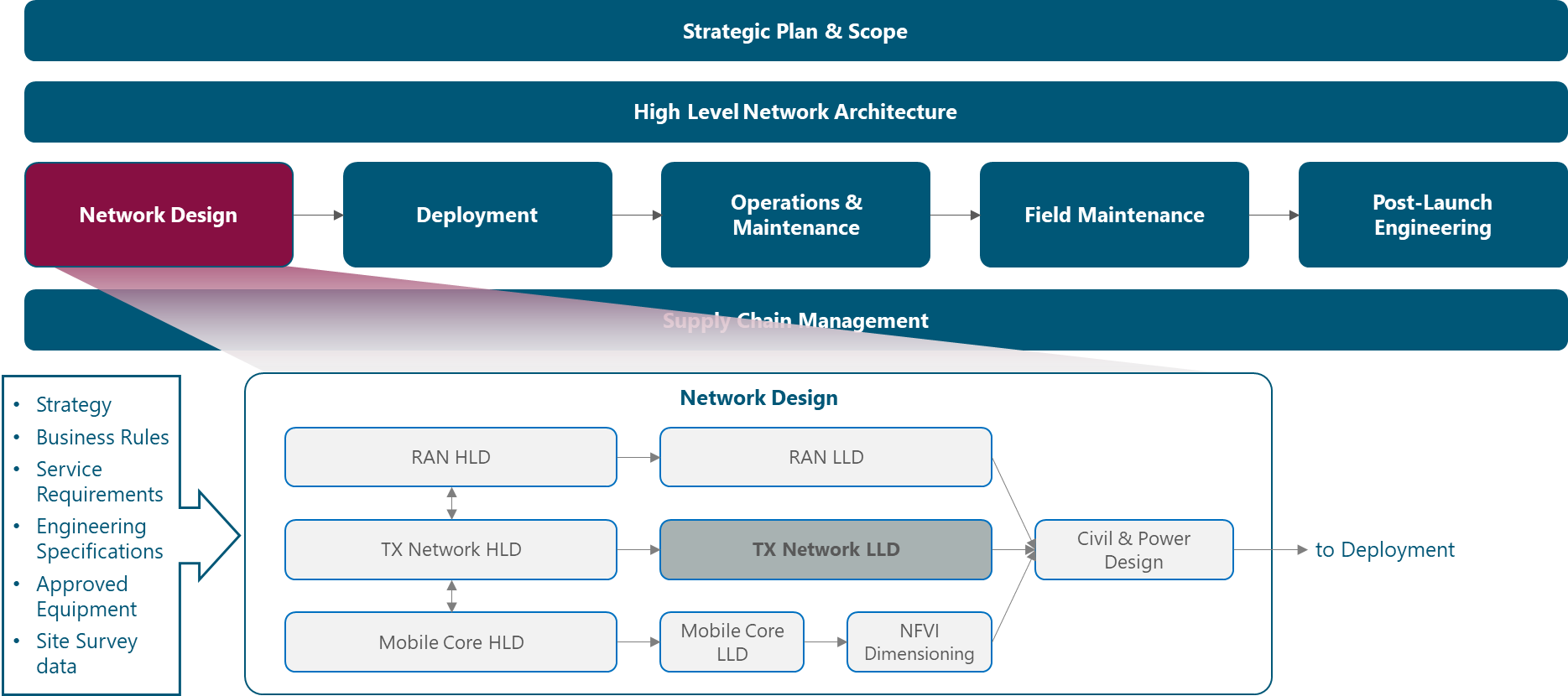
Figure 1. Module Framework
Figure 2 presents the Tx Network LLD functional view where the main functional components are exhibited. Critical module inputs are further described and examined in Section 2.2. In addition, guidance and methodologies to execute the tasks included within each function are described in Section 3.
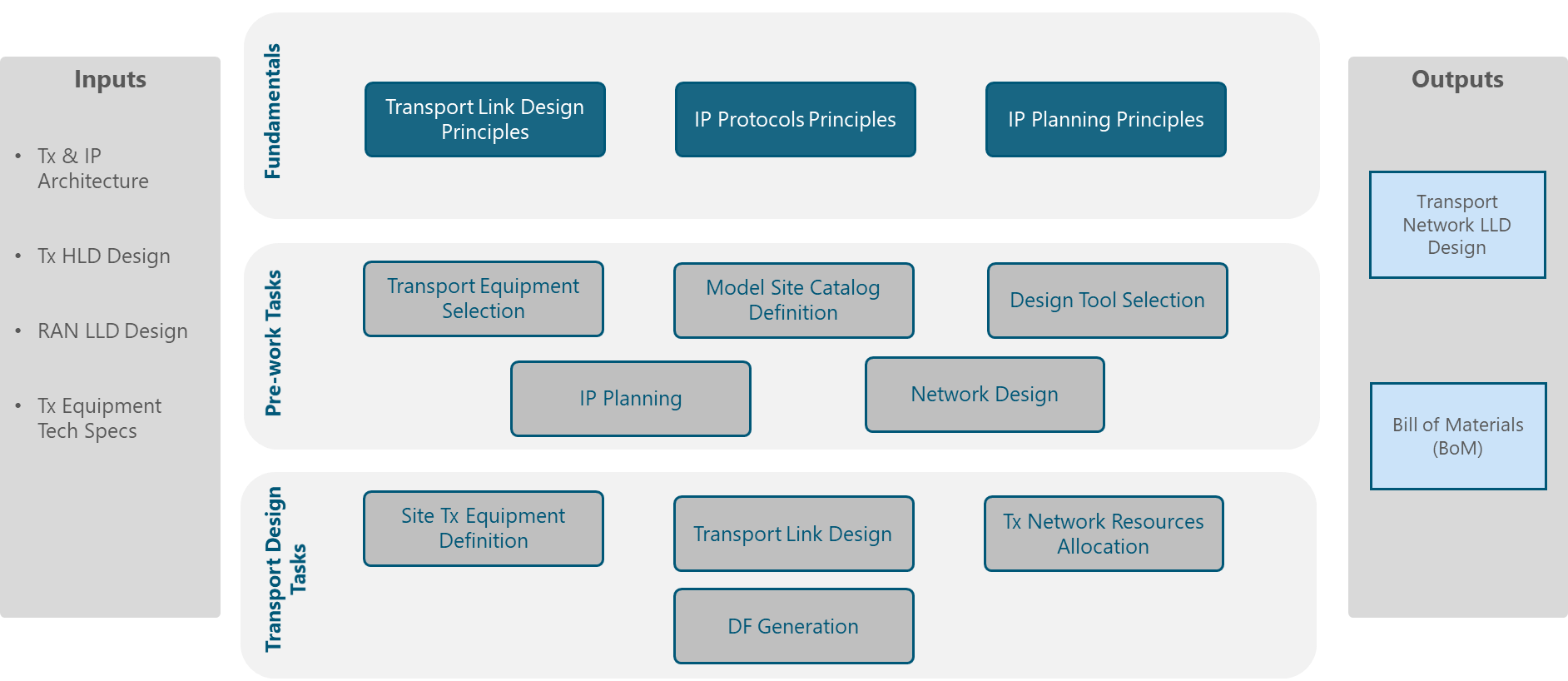
Figure 2. Module Functional View
The rest of the module is divided into four sections. Section 2 is a birds-eye view of the Tx network fundamentals involved on its design. Once fundamental knowledge is acquired, Section 3 focuses in showing a hands-on view of the tasks involved on the design. Section 4 organizes functional tasks on an end-to-end process flow that can be used as-is or be adapted by NaaS operators to match with their particular conditions. Finally, Section 5 illustrates how to integrate previous elements into a comprehensive Low-level Design (LLD) recommendation.
2 LLD Fundamentals
This section provides a general overview of the baseline concepts to develop a Tx Network Low-level Design.
2.1 Tx Network Environment
In a mobile environment, the Transport Network interconnects different networks including the RAN (Radio Access Network), data centers and external networks. Figure 3 displays the architecture of a typical transport network.
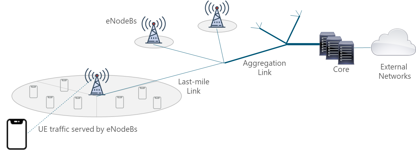
Figure 3. Typical Transport Network
Mobile networks are ubiquitous and support a mix of different types of traffic originating from and terminating to mobile devices. All this traffic must be conveyed between the mobile cellular base stations through the transport network up to the Mobile Core. For this reason, different aggregation levels exist on the transport network which for most of NaaS Operators can be classified as: last-mile and aggregation level.
The implementation of 4G Long-Term Evolution (LTE) imposes some requirements on transport networks such as more network capacity and latency reduction. These requirements are better served through terrestrial technologies (fiber optic and microwave). However, in rural areas, this becomes a challenge because satellite transport is usually the only feasible technology. For this reason, transport network infrastructure is an essential component of the NaaS Operator network and its design must be performed with optimal processes and techniques
2.2 Tx Network Low-level Design Inputs Description
This section analyzes the module input data and their respective candidate sources, which is presented in Table 1. Furthermore, the impact of module inputs on the design process is examined.
|
Input Required |
Description |
Candidate Source |
Impact |
|
Tx & IP Architecture |
Includes the technologies and protocols to be considered on the design |
Tx & IP Architecture Module |
– Establishes the available transport technologies to be designed and their respective design guidelines. |
|
Tx HLD Design |
Describes the High-level Tx solution (transport technology, transport nodes) |
Tx HLD Module |
– The type and total number of Tx Links to be designed determines the selection of the tool to perform the Tx Link Design. |
|
RAN HLD Design |
Describes the parameters related to RAN solution (site location, RAN equipment, covered population) |
RAN HLD Module |
– The RAN equipment model has a direct impact on the Model Site Catalogue generation |
|
Transport Provider Network Data |
Contains specific information regarding Tx nodes (name, IP addresses, Port, S-VLAN) |
Transport Provided Network Database |
– The specific data of the Transport Node is used during the Datafill generation process. |
|
Tx Equipment Technical Data |
Contains a List of candidate Tx equipment for all involved vendors. |
Tx Equipment Vendor |
– Establishes the Transport (Transmission and IP) Equipment to be evaluated. This has a direct impact on Transport Equipment Selection and Model Site Catalogue generation. |
|
General IP Address Distribution |
Defines the general segments for transport equipment and services. |
Tx & IP Architecture Module |
– The General IP Address Distribution is used on IP Planning and Tx Network Resources Allocation steps. |
Table 1. Tx LLD Module inputs analysis
2.3 Tx Link Design
Transport links are subject to multiple phenomena (e.g. meteorological) that have a direct impact on the link performance. Therefore, an accurate Tx Link Design must be performed to ensure that the transport link will behave within the performance thresholds under different conditions.
This process must be performed individually for each transport link according to the engineering guidelines from Transport & IP Architecture. Furthermore, this process uses specialized link design tools (See Section 4.2.3 for further details) that consider additional parameters (e.g. weather conditions) and their impact on the transport link performance. Each transport technology has its particular parameters that must be calculated in order to maintain the transport link operating in optimal conditions.
Tx Link Design for Fiber and Microwave technologies is perform within this module to validate the site feasibility, and confirm physical and logical parameters. In, contrast, for Satellite technology, the most common implementation scenario is to use a Satellite Service provider and this validation is determined by the satellite footprint. Furthermore, the detailed Satellite Link Design is performed by the Satellite Service provider and is included as part of the equipment delivery.
2.4 Network Design
The most common implementation scenario implemented in the transport network is displayed in Figure 4:
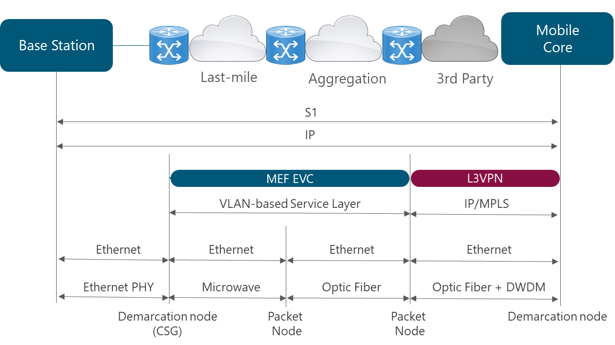
Figure 4. Transport network scenario based on Carrier Ethernet with L3VPNs
In order to support the scenario presented in Figure 5, NaaS operators must define the different protocols and technologies to be used at different layers.
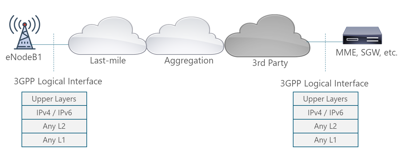
Figure 5. 3GPP Logical Interfaces Protocol Stack
The definition of the stack protocols to be implemented is an input from the Transport & IP Architecture Module. The scope of the LLD process is to define the main configurations parameters for each of them.
2.5 IP Planning
In order to simplify the IP address management of the overall network, support several technologies and be able to perform an efficient troubleshooting, an IP Address Distribution Plan must be defined. An IP Address Distribution Plan is a document developed by the NaaS Operator that displays how the universe of available IP addresses will be distributed in a way that supports the required services. This plan should satisfy the following conditions:
Section 3.3 details the methodology to generate the Detailed IP Distribution Plan and the IP Address Allocation process using IPv4 version. A similar process can be performed when using IPv6 version considering that 16 octets are available. A broader view on the fundamentals of this process can be found on the Primer on IP Planning Principles.
3 Functions & Methodologies
Methodologies to perform critical tasks/subtasks involved in the Tx Network Low-level design process.
3.1 Fiber Optic Link Design
This section provides general methodologies to perform the Passive Fiber Optic Link Design. The inclusion of active elements in the fiber path (e.g. amplifiers) is out of the scope of this module.
3.1.1 Fiber Optic Link Design Process
A Fiber Optic Link Design must be developed for each of the fiber paths defined by the Tx High-Level Design in order to complete the Tx information. The principal analysis is the Fiber Optic Link Budget, which is the verification of a fiber optic link operating characteristics. This encompasses items such as routing, circuit length, fiber type, number of connectors and splices and wavelengths of operation.
Although the specific steps can vary depending on the selected Fiber Optic Link Design Tool, the general steps to perform the Fiber Optic Link Budget are presented in the following subsections.
Step 1. Load Fiber Optic Equipment Characteristics
The information regarding the Fiber Optic Equipment that can be included depends on the selected tool characteristics. However, the following elements are the most relevant in the Fiber Optic Link Design:
Figure 6 shows an example of the configuration of the Fiber Optic Equipment Characteristics in the Fiber Optic Link Design Tool.
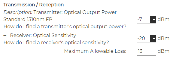
Figure 6. Example of Fiber Optic Equipment Characteristics in Fiber Optic Link Design Tool.
Step 2. Calculate the Losses in the Fiber Path
The information regarding multiple losses in the fiber path that can be included depends on the selected tool. However, the following elements are the most relevant in the Fiber Optic Link Design:
In absence of specific values, the use of conservative defaults is advisable, as noted in Table 2:
|
Wavelength |
Fiber Loss / km |
Connector Loss |
Splice Loss |
|
1310 nm |
0.35 dB |
0.75 dB |
0.3 dB |
|
1550 nm |
0.22 dB |
0.75 dB |
0.3 dB |
Table 2. Default values for Link Budget Calculations
The total loss in the optical link is thus computed, using a typical safety margin or 3dB, as:
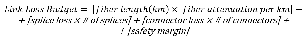
(Eq. 1)
Figure 7 shows an example of the configuration of the Fiber Losses in the Fiber Optic Link Design Tool.
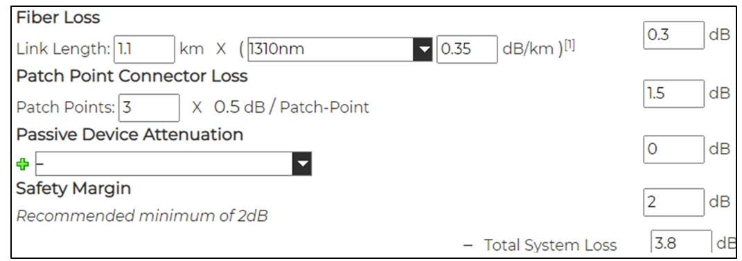
Figure 7. Example of Fiber Losses in Fiber Optic Link Design Tool.
Step 3. Fiber Optic Link Budget Generation.
A link budget is a calculation that considers the transmitted power with all the gains and losses in the Tx link in order to estimate the strength of the received signal. This calculation provides, for a link Loss Budget and a given dynamic range (the difference between the transmitter power and the receiver sensitivity) the adjustment margin for that configuration as:
![]()
(Eq. 2)
Per design, the power margin should be greater than 3dB. The Fiber Optic Link budget is calculated by using the options provided by the selected tool.
Step 4. Fiber Optic Link Requirements Validation
In order to validate the Fiber Optic link design, the Link Budget must be fulfilled (i.e. it must confirm that the power margin is greater than 3dB).
In case the Link Budget is not fulfilled, a change in the link parameters can be modified (e.g. change the transmission power) as long as the link still complies with design directives.
3.1.2 Fiber Optic Link Design Report
After generating the Fiber Optic Link Design, a report that contains information of the designed link must be constructed including the following information:
3.2 MW Link Design
This section provides general methodologies to perform the Tx Link Design for each available MW Link identified in the High-Level Design based on the established requirements.
3.2.1 MW Link Design Process
Although the specific steps can vary depending on the selected Microwave Link Design Tool, the general steps to perform the Microwave Link Design are presented in the following subsections. It is worth to note that the illustrative images along the process belong to Pathloss Tool.
Step 1. Digital Terrain Databases Selection
In general, most propagation predictions are based on detailed topographical information. The topographical information is provided by Digital Terrain Elevation (DTE) Models that is composed by digital terrain topographical databases and represented in the form of digital terrain maps. These models provide accurate information that will be used to evaluate the path clearance and the potential loss associated with diffraction.
Depending on the selected tool to perform the design operations, these DTEs models can be included as part of the tool. If they are not included, some DTEs are available as open source data for many places in the world (e.g Google Maps Elevation API).
Figure 8 shows an example of the configuration of the Digital Terrain Database in the MW link Design Tool.
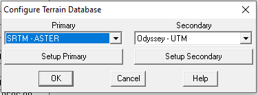
Figure 8. Example of Digital Terrain Database Configuration on MW Link Design Tool.
Step 2. Load Site Information
The site information must be introduced to the tool, including:
Figure 9 shows an example of the configuration of the Site Information in the MW link Design Tool.
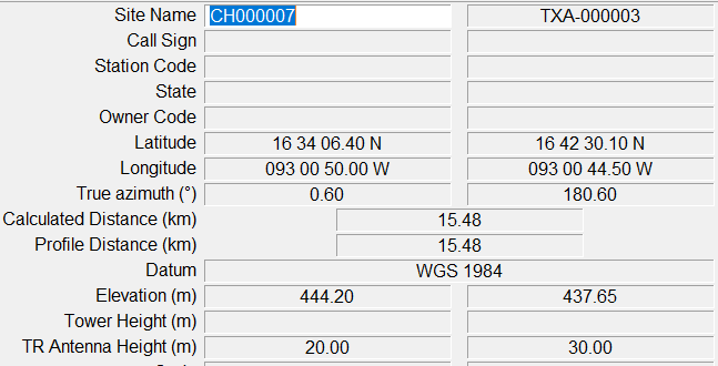
Figure 9. Example of Site Information Configuration on MW Link Design Tool.
Step 3. Load MW Equipment Specifications
The information regarding the MW equipment that can be included depends on the selected tool features. However, the following elements are the most relevant in the MW Link Design:
Furthermore, depending on the tool, this information may be entered via a user interface or equipment files (e.g. MRS files in Pathloss). Figure 10 shows an example of the configuration of the MW Equipment in the MW link Design Tool.

Figure 10. Example of MW Equipment Configuration on MW Link Design Tool.
Step 4. Additional MW Link Model Characteristics Setting
Depending on the selected tool features, additional Microwave Link Model Characteristics can be configured, such as:
Step 5. MW Link Budget and Profile Generation
Generate the Microwave Link budget and profile using the options provided by the selected tool. Figure 11 displays an example of a MW Link Profile.
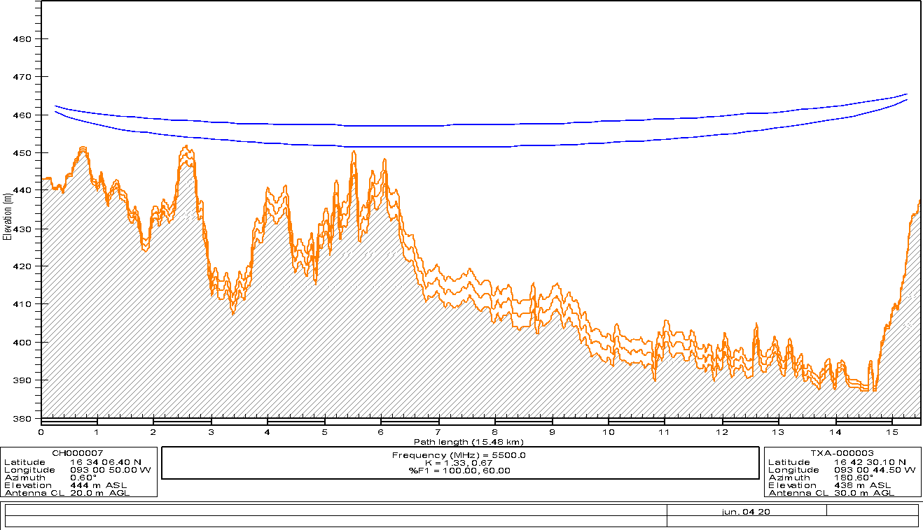
Figure 11. MW Profile Example
Step 6. MW Link Requirements Validation
All the MW links must comply with the general requirements established in the Tx & IP Architecture module as well as with the specific MW link parameters (e.g. availability, throughput). In case one of the requirements is not fulfilled change in the link parameters can be applied as long as the link still complies with the design directives.
For instance, if the received signal strength do not surpass the radio sensitivity, a lower modulation scheme can be selected. This change, inherently increase the radio sensitivity, allowing to receive weaker signals. However, a change in the modulation scheme may impact in the link throughput.
Furthermore, in case the link is not feasible due to lack of Line of Sight (e.g. no Line of Sight due to an insuperable obstacle), the methodology presented in Section 3.2 of Tx HLD Module must be applied to re-design the MW Link.
3.2.2 Microwave Link Design Report
After generating the MW Link Design, a report that contains information of the designed link must be constructed including the following information:
Figure 12 displays an example of the Microwave Link Design Report generated by the Pathloss tool.
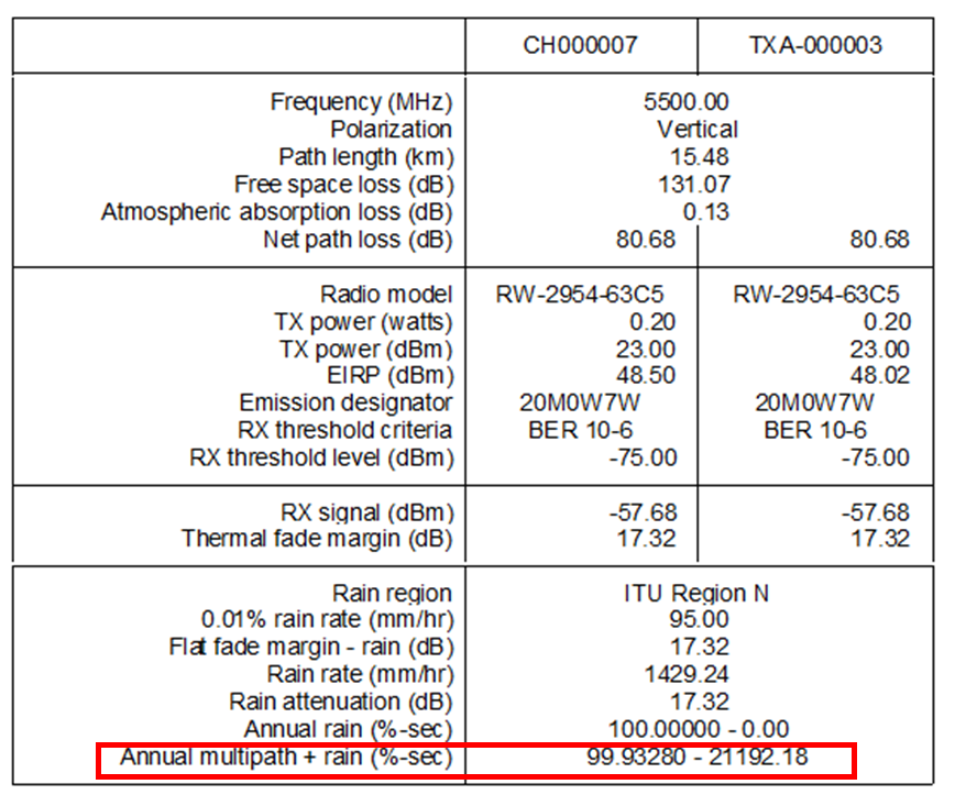
Figure 12. MW Link Report Example
3.3 IP Address Subnetting Process
IP Subnetting is the process used to partition a network address space into smaller segments (e.g. divide one segment /8 into 16 segments /12). This process is important in the context of the NaaS operator because it allows to logically divide the network traffic type for different uses (e.g. separate the traffic of the eNodeBs from the Core elements). Furthermore, IP Subnetting allows to use different masks for each subnet, and thereby use address space efficiently. Finally, subnetted networks are much easier to manage and troubleshoot.
In order to illustrate the process, a practical Example is followed along each of the processes steps. In this particular example, the process to divide the segment 10.0.0.0/16 in appropriate network subnets that can allocate the number of IP addresses in Table 3 is presented.
| |
Number of required IP addresses |
|
Subnet 1 |
20,000 |
|
Subnet 2 |
10,000 |
|
Subnet 3 |
15,000 |
Table 3. IP Address Requirements in Subnetting Example
Step 1. Calculate the required block sizes
In order to calculate the length mask (i.e. block size) required to support the number of required IP addresses, the following formula is used:
![]()
(Eq. 3)
Using Eq. 3 in the example, the results presented in Table 4 are obtained. In practice, the assign block size must be greater than the actual requirement. A Web-based IP address Calculator tool can be used to simplify the planning on network subnets.
|
Subnet |
Required Mask Length |
Mask Notation |
Block Size |
|
Subnet 1 |
/17 |
255.255.128.0 |
32,768 |
|
Subnet 2 |
/18 |
255.255.192.0 |
16,384 |
|
Subnet 3 |
/18 |
255.255.192.0 |
16,384 |
Table 4. Block size Requirements in Subnetting Example
Step 2. Subnet Sorting
The next step is to sort the resulting network segments based on the block size in descending order. In this way, the IP address space is used efficiently. In some cases, it is possible that the sum of the calculated block for the required subnets, does not make complete use of the available IP segment. These additional IP addresses can be reserved for future expansion.
It is important to note that the subnetting definition process must consider future additional network elements. Further changes in the existing subnets definition are difficult and can result in the modification of the IP Distribution Plan. It is recommended to be conservative in the calculation of the required block sizes to reduce the likelihood of having to re-work on the IP subnetting process.
Step 3. Subnets Assignment
Finally, assign the first resulting network segment to the first available segment from the original segment and continue following the ordering. The Example Result is displayed in Table 5.
|
Subnet |
Required Mask Length |
|
Subnet 1 |
10.0.0.0 / 17 |
|
Subnet 2 |
10.0.128.0 / 18 |
|
Subnet 3 |
10.0.192.0 / 18 |
Table 5. IP Subnetting Result in Subnetting Example
Additionally, Naas operators can use the High Level IP Distribution Plan Widget as support in the generation of the IP Distribution Plan.
3.4 IP Address Allocation
IP Address Management is the collection of procedures for organizing, tracking and adjusting the information related to the IP addressing space. It supports the network designers and operators to guarantee that the IP addresses remain updated. Furthermore, given the possible thousands of IP addresses in the network, this process also helps the operations team when debugging / troubleshooting issues.
Although the specific steps can vary depending on the selected IP Address Management Tool, the general steps to perform the IP Address Allocation are presented in the following subsections. It is worth to note that the illustrative images along the process belong to the free phpIPAM Tool.
Step 1. Define Network Segments
Introduce the main network segments included in the General IP Distribution Plan in descending order of block size. Then introduce all the network segments included in the Detailed IP Distribution Plan.
Step 2. Allocate IP Network Addresses
To allocate a specific IP address (e.g. for eNodeB services or transport equipment), identify the segment that corresponds to the scenario in the Detailed IP Distribution Plan.
Once the specific segment is identified, the first available IP address within the segment is selected, and the specific information is introduced to describe the segment purpose. Following the basic information that must be registered for all the IP addresses within the IPAM Tool:
Figure 13 displays an example of the IP Allocation in the phpIPAM tool.
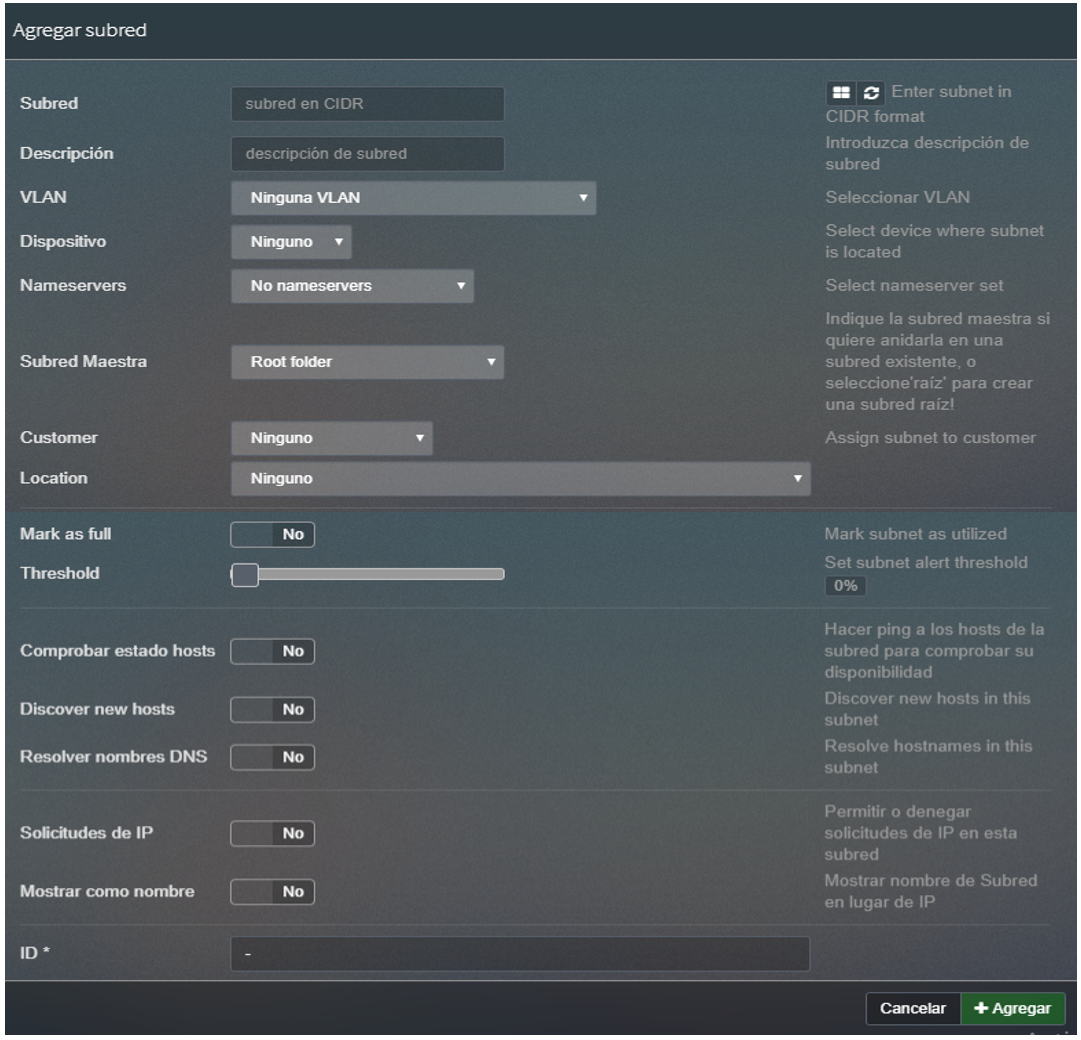
Figure 13. Subnet Allocation Example
4 E2E Process Flow
This section presents a generic yet customizable end-to-end process flow to perform the transport design for the transport network.
4.1 End-to-end Process Overview
The generic end-to-end (E2E) process flow displayed in Figure 14 orchestrates general tasks to perform the Transport Network LLD in a logical and well-structured sequence.
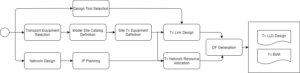
Figure 14. Generic E2E Process Flow.
Details and customization options of each step are reviewed in the following sections. In addition, a Tx LLD Process Flow Designer is provided as part of the Methods of Engagement.
4.2 Step-by-step Analysis
This section presents an examination of each of the steps involved in the Low-level Tx Design process to identify, isolate and describe the range of implementation options on the path towards customization based on NaaS operator requirements and constraints.
In order to demonstrate a practical exercise to implement the process design flow, a Design Example is followed along each of the process steps.
Design Example
In this particular example, the process to generate the LLD Design for the scenario in Figure 15 is presented. It must be noted that this is the continuation of the Example presented in the Tx HLD Design.
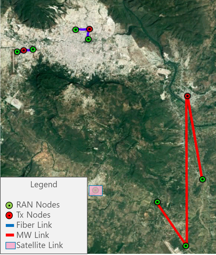
Figure 15. Design Example Scenario.
The scenario is composed of eight RAN sites that will be analyzed to perform the Transport LLD Design. The example considers two geographical regions (North and South), where all the RAN sites presented are located in the North Region.
The distribution of transport technologies is the following: Four nodes use Fiber Optic, three nodes use Microwave and one site uses Satellite Link. The details on the transport technologies selection can be found in the Tx HLD Module.
The General IP Distribution Plan is presented in Table 6. The General IP Distribution Plan is presented in Table 6, and it describes the general segments defined by each of the different network elements. The details on the General IP Distribution Plan generation can be found in the Tx & IP Architecture Module.
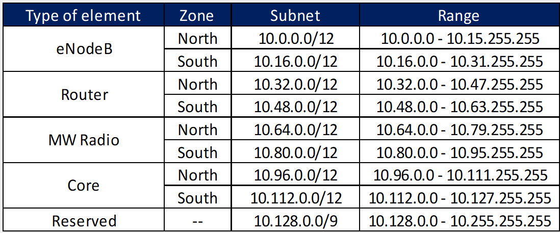
Table 6. General IP Plan Distribution for the Example Scenario.
The VLAN Definition to be used to separate the traffic for different planes is presented in the Table 7. The details on the VLAN Definition can be found in the Tx & IP Architecture Module.
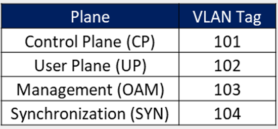
Table 7. VLAN Definition in Design Example.
Whereas this Design Example only focuses on the eight RAN sites presented in Figure 15, the total number of expected RAN sites and Tx links to be deployed are presented in Table 8. These numbers already consider the future growth of the network.
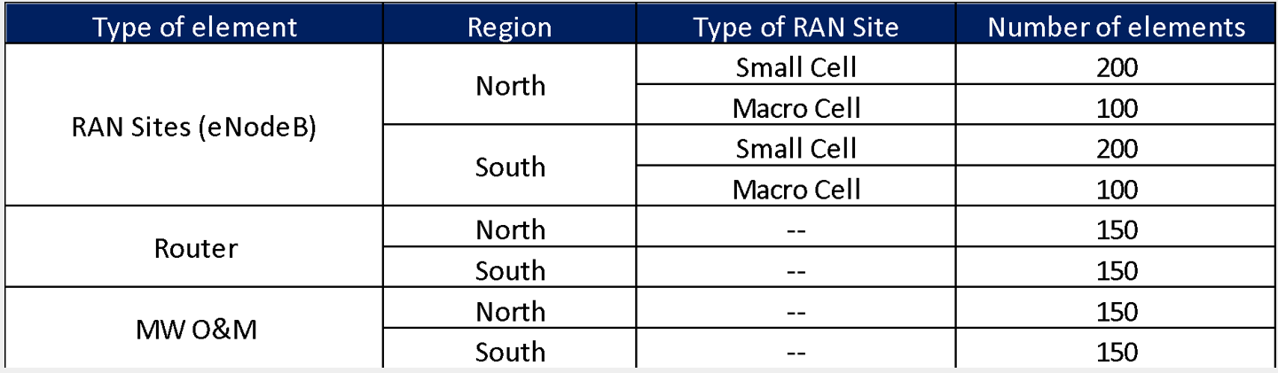
Table 8. Total number of elements for the Example Scenario
Even if the number of required IP addresses for the number of elements does not cover in totality the corresponding IP segment, the methodology presented in Section 3.3 must be performed to enhance the network management and support future expansions.
4.2.1 Transport Equipment Selection
NaaS operators must perform the selection of the Tx Equipment from multiple vendor alternatives. The complete process to select the Tx Equipment is included within the Procurement Module (RFx Process Module). This section focuses on the technical aspects to perform the evaluation of transport equipment from different vendors.
From the technical perspective, Table 9 displays the typical requirements that the transport equipment must satisfy which must be defined according to the required network segment (e.g., last-mile or aggregation link implementation scenario).
|
|
|
|
Supported Protocols |
Support for the protocols defined in Tx & IP Architecture Module |
|
Availability |
Reliability and uptime |
|
Time-to-Repair |
|
|
Time-to-Deploy |
|
|
Performance |
Throughput performance under normal and stressing conditions |
|
Maximum number of active connections |
|
|
Dimensions |
Standard dimensions compliance |
|
Power Requirements |
Type of energy required (AD/DC) and power consumption profile |
|
Security |
Implemented security mechanisms |
|
Cost |
Cost of the equipment. |
Table 9. Typical specifications to be evaluated in transport equipment.
>
The decision to select the Tx Equipment is also affected by the financial constraints of the project. The final selection of the Tx Equipment is performed during the RFx process and in conjunction with the Procurement Team.
Design Example
In the Design Example, there are two Tx equipment provided by different vendors (Vendor A and Vendor B) that are evaluated for selection. The characteristics of the Tx equipment are shown in Table 10.
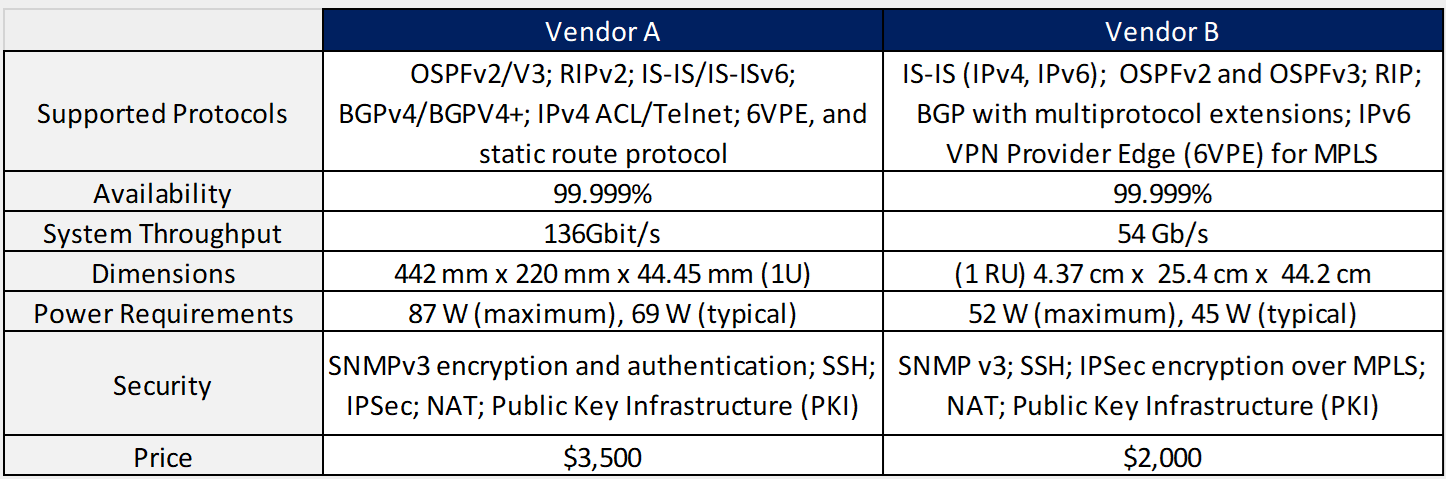
Table 10. Tx Equipment Specification for Design Example.
From Table 10, it can be seen that both options comply with the required protocol stack and security features; they also have a similar value of the availability figure and both require a standardized unit rack for installation. Vendor A offers more system throughput, but it also has more power requirements and the price is considerably higher.
Therefore, Vendor B is the selected option in the Design Example since it complies with the required protocol stack, security features, system throughput (it fully complies with the architecture requirement). Furthermore, the power requirements are low (a critical aspect in rural environments) and the price is the most accessible.
>
4.2.2 Model Site Catalogue Definition
The aim of Model Site Catalogue Definition is to standardize and document the possible Tx Site equipment configurations to be implemented. By doing this, the design options are constrained which simplifies the overall process.
4.2.2.1 Model Site Granularity Definition
In order to create the catalogue, the granularity to be used must be defined. Granularity is the level of detail present in the scenarios included in the catalogue and will dictate the different variations to be included in the catalogue. The possible alternatives to be used to establish the granularity are:
NaaS operator should select the appropriate level of granularity that better suits its requirements. However, it is highly recommended that a high level of granularity is chosen in order to minimize the number of possible alternatives and simplify the design process.
4.2.2.2 Model Site Catalogue Generation
Based on selected granularity, an identification of all possible scenarios is performed. Then, a high-level description of each scenario solution must be described. Following, a list of characteristics that must be identified for each scenario:
Figure 16 displays a brief example of the Model Site Catalogue Generation considering Available Transport Technologies and Tx Equipment Vendor as granularity. NaaS operators can take this example to customize its own catalogue generation process.
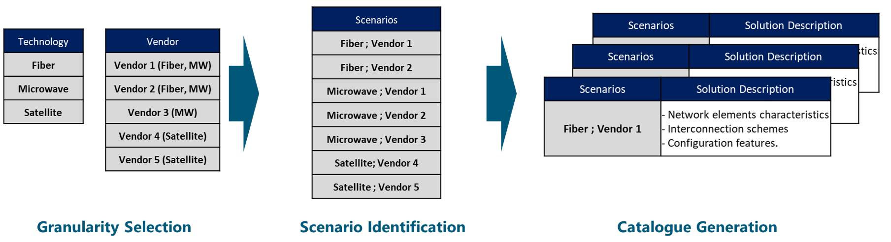
Figure 16. Example of Model Site Catalogue Generation
The NaaS Operator can use the Model Site Catalogue Template as a base to create its own version.
Design Example
In order to generate the Model Site Catalog Standard Configurations for the transport equipment on the Design Example, the following scenarios are identified:
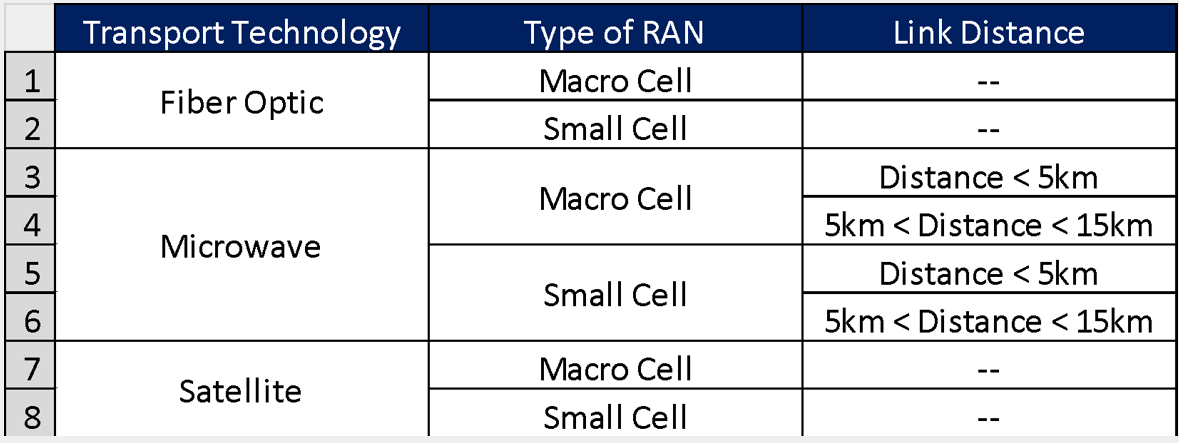
Table 11. Model Site Catalogue Scenarios for Design Example.
Figure 17 illustrates the site topology of the scenario: Microwave Macro Cell.
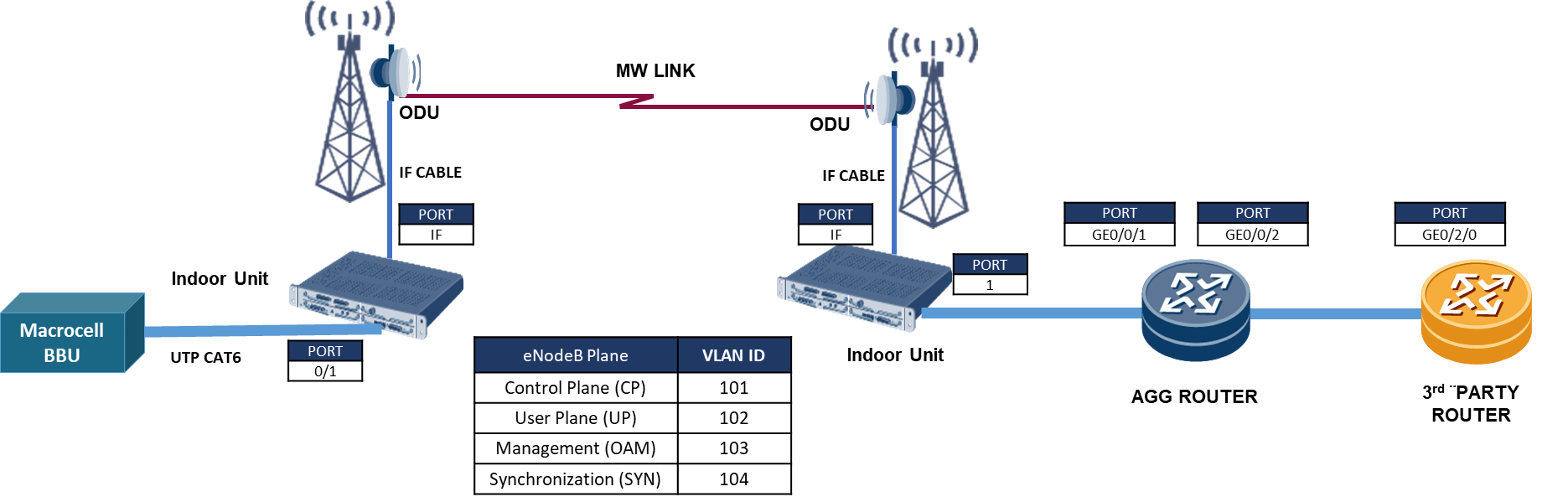
Figure 17. Site Topology Scenario for Design Example
4.2.3 Design Tool Selection
This section provides general criteria for the selection of the most suitable set of tools and level of automation to be implemented during the design phase.
In order to select the appropriate design tools to perform the Transport LLD, a classification of available tools is required. Table 12 displays a generic tool type classification that will serve as a base to perform the selection.
|
Tool Type |
Implementation type |
Type of License |
Automation |
Customization |
Support Type |
|
Tier 1 |
Commercial tool |
License cost |
High/Medium: Batch mode usually based on scripts |
High: Customization options provided by developer |
Dedicated support (extra charges can apply) |
|
Tier 2 |
Open-source code |
Free |
High/Medium: Batch mode usually based on scripts |
Medium/High: Customization options implemented by users |
Wiki + Community Groups |
|
Tier 3 |
Web-based, APIs |
Free (sometimes usage limited per day) |
Low: Usually, one by one approach |
Low: Usually only proprietary parameters are defined |
Limited support |
|
Tier 4 |
Home-grown (e.g Spreadsheet) |
Free |
Medium: Automation options requires high cycle times |
Medium: Customization options requires high cycle times |
No support |
Table 12. Tool Type Classification
>
For each type of design tool consider in the design process, there are multiple available options that are examined in the following subsections.
4.2.3.1 Tool Selection Process
The selection process must consider different aspects regarding the scope of the project and the characteristics of the NaaS operator, following a list of examples:
Figure 18 displays a generic process to perform the Tool Selection. NaaS operators can use this process as a base to define its own version according to operators priorities.
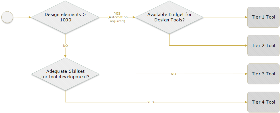
Figure 18. Tool Selection Process
4.2.3.2 Fiber Link Design Tool Selection
The tools utilized to perform the Fiber Link Design are classified in Table 13 according to the parameters defined.
|
Tool Type |
Name |
Description |
|
Tier 1 |
VPItransmissionMaker – VPIphotonics |
Fiber Link Design Tool based on graphical interface, a robust simulation scheduler and realistic simulation models |
|
Tier 3 |
Optical Power Budget Calculator – Evert |
Optical Power Budget Calculator available through a web-based interface. |
Table 13. Tool Classification for Fiber Optic Link Design
>
Following the methodology presented in Section 4.2.3.1, the NaaS operator can perform the selection of the Fiber Link Design Tool.
Design Example
The tool Optical Power Budget Calculator – Evert will be used as GIS Tool to perform the Fiber Path Design in the Design Example.
>
4.2.3.3 Microwave Link Design Selection
The tools utilized to perform the Microwave Link Design are classified in Table 14 according to the parameters defined.
|
Tool Type |
Name |
Description |
|
Tier 1 |
Pathloss |
The Pathloss program is a comprehensive Microwave Radio Link Design and Planning Software for radio links operating in the frequency range from 30 MHz to 100 GHz. |
|
Tier 3 |
Link Budget Calculator – Radwin |
MW Link Design Tool available through a web-based interface. It only uses proprietary equipment. |
Table 14. Tool Classification for Microwave Link Design
>
Following the methodology presented in Section 4.2.3.1, the NaaS operator can perform the selection of the Microwave Link Design Tool.
Design Example
The tool Pathloss will be used as a Microwave Link Design Tool to perform the link budget generation in the Design Example.
>
4.2.3.4 IP Address Management
The tools utilized as IP Address Management are classified in Table 15 according to the parameters defined.
|
Tool Type |
Name |
Description |
|
Tier 1 |
IP Address Manager – Solarwinds |
IPAM Tools with integrated DHCP, DNS, and IP address management. |
|
Tier 2 |
phpIPAM |
Open-source web IPAM Tool. It is php-based application with MySQL database backend, using jQuery libraries, ajax and HTML5/CSS3 features. |
|
Tier 4 |
Excel-based IPAM |
Home-grown IPAM bases on Excel spreadsheets. |
Table 15. Tool Classification for IP Address Management
>
Following the methodology presented in Section 4.2.3.1, the NaaS operator can perform the selection of the IP Address Management Tool.
Design Example
The tool phpIPAM will be used as an IP Address Management Tool in the Design Example.
>
4.2.4 Network Design
The configuration process for each network protocol varies depending on the equipment vendor. However, it is important that all network elements have its parameters set with the same guidelines to avoid inconsistencies that may potentially cause service degradation.
The different characteristics that need to be defined for each layer are examined in the following subsections.
4.2.4.1 L1 / Physical Interfaces
This layer is concerned with the transmission and reception of the unstructured raw bit stream over a physical medium. Therefore, it defines the characteristics of the physical interfaces that will be consider in the deployment phase.
It is highly recommended that all the transport equipment support transceiver modules based on small form-factor pluggable (SFP). In this way, the interface port can be equipped with any suitable type of transceiver as needed.
Ethernet supports both electrical (twisted-pair cable) and optical fiber interfaces for physical connection. The electrical interfaces are recommended for connections between co-located equipment, this means equipment that are physically on the same Location (e.g in the same site, equipment room). In this case, the maximum distance allowed for electric interfaces is 100m.
Table 16 displays the typical selection for the physical interfaces to be implemented in transport networks:
|
Transceiver Module |
Media |
Interface Type |
Distance Range |
|
|
1G |
SPF |
Electrical |
1000BASE-T |
100m |
|
Optical |
1000BASE -LX10 |
10km |
||
|
10G |
Electrical |
10GBASE-T |
75m (100m with cable Cat6a) |
|
|
Optical |
10GBASE -LR |
10km |
Table 16. Typical values for physical interfaces.
>
4.2.4.2 L2 / Data Link Layer
For the L2 Layer, the majority of LTE mobile equipment utilize Ethernet interfaces for transport, therefore, Ethernet based services are most suitable to be implemented in the transport network.
Table 17 displays the basic configuration information to implement the Ethernet protocol in the network.
|
Parameter |
Description |
Criticality |
Comments |
|
Maximum transmission unit (MTU) |
Largest size packet that can be processed by nodes within the transport network. |
Mandatory |
Configure the MTU definition from Architecture module consistently in all network equipment |
|
Group Member |
Group of interfaces in LAG |
Optional |
Only in LAG configuration. |
|
Description |
Includes information regarding the use of the interface |
Optional |
Must contain self-explanatory information |
Table 17. Ethernet Protocol Basic Configuration
>
Finally, Table 18 displays the typical configuration for the VLAN parameters.
|
Plane |
VLAN Tag |
|
Control Plane (CP) |
101 |
|
User Plane (UP) |
102 |
|
Management (OAM) |
103 |
|
Synchronization (SYN) |
104 |
Table 18. Typical VLAN configuration
>
4.2.4.3 L3 / Routing Layer
The L3 Routing layer controls the physical path the data should take based on network conditions and other factors. Figure 19 displays a typical implementation for L3 Routing protocols. More detail regarding the selection of these protocols can be found in the Transport & IP Architecture Module.
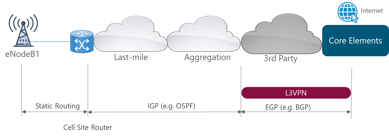
Figure 19. Typical L3 Routing Protocol Implementation
The following subsections examine the basic configuration parameters to implement the displayed network routing mechanisms. However, the required transport protocols are defined in the Transport & IP Architecture Module.
Static Routing
Static routes define explicit paths between two routers and cannot be automatically updated. Its configuration is simple as for each static route it is only needed to specify the egress interface and optionally, the next-hop address.
The static route is only recommended to be used on endpoints where a single connection is available. For instance, in a scenario where only one Cell Site Router is deployed, the eNodeB can only send the traffic to this element.
OSPF Protocol
The Open Shortest Path First (OSPF) protocol is a link-state routing protocol that uses a hierarchical routing model where a centralized routing domain is defined within an autonomous system. OSPF can be used in the aggregation domain when more complex topologies are presented.
Table 19 displays the basic configuration information to implement the OSPF protocol in the network.
|
Parameter |
Description |
Criticality |
Comments |
|
Process ID |
Used to differentiate multiple OSPF processes on the same router. |
Mandatory |
Any number from 1 to 65,535 |
|
Interface |
Specify the interfaces included in the OSPF process. |
Mandatory |
According to device configuration (See Model Catalogue) |
|
Area |
Limit the scope of route information distribution. |
Mandatory |
The default area is 0.0.0.0 |
|
Network |
Identify which device interface will be included within the OSPF process. |
Mandatory |
Should be configured based on the IP Distribution Plan for each network device |
|
Retransmit interval |
Specifies the interval between link-state advertisement (LSA) retransmissions for adjacencies belonging to an OSPF interface |
Optional |
5 sec |
|
Authentication Method |
Used to protect the router from unauthorized OSPF peering connection. |
Mandatory |
Security will be use MD5 password. |
Table 19. OSPF Protocol Basic Configuration
>
BGP Protocol
The Border Gateway Protocol (BGP) is a distance vector that is used to advertise the route prefixes outside the organizational boundary without revealing the internal routing characteristics. BGP is commonly used to exchange prefixes assigned to mobile subscribers to the providers Internet peer.
Table 20 displays the basic configuration information to implement the BGP protocol in the network.
|
Parameter |
Description |
Criticality |
Comments |
|
AS Number |
Identified the AS domain. |
Mandatory |
Deploy BGP under Private AS number 65535 |
|
Router ID |
Used to identify BGP-speaking peers. |
Mandatory |
Set the BGP router ID with loopback 0. |
|
Neighbor |
Configure the relationships between BGP speakers. |
Mandatory |
Should be configured based on the IP Distribution Plan for each network device |
|
Authentication Method |
Protect the router from unauthorized connection. |
Mandatory |
Security MD5 authentication will be implemented in all sessions. |
Table 20. BGP Protocol Basic Configuration
>
4.2.4.4 L4 / Transport Layer
The most commonly used transport layer protocols are:
These protocols do not need additional configuration to be used.
Design Example
The Basic Configuration presented for each of the network layers is considered in the Design Example.
In particular, for Layer 3 protocols, the configuration used in the Design Example is presented in Table 21
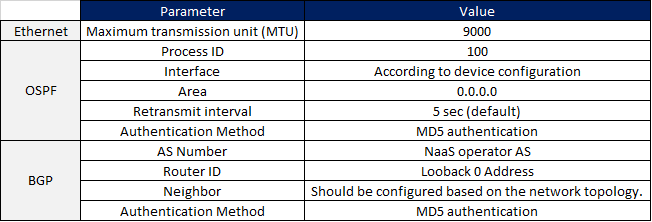
Table 21. L3 Protocol Configuration in Design Example.
>
4.2.5 IP Planning
This section describes the guidelines to perform the calculation of the required IP resources to implement the Transport LLD Design and generate the Detailed IP Distribution Plan. The General IP Distribution Plan is an input provided by the Tx & IP Architecture Module.
The Detailed IP Distribution Plan should cover the anticipated growth in the number of network elements in order to avoid frequent changes. Furthermore, it should allow summarizing routes in the network. This optimizes routing performance and avoids a large memory consumption in the routers.
Step 1. Scenarios Identification
For each of the main segments in the General IP Distribution Plan, an identification of all of the possible segmentation criteria must be performed. In order to maintain the IP distribution Plan simple, it is recommended to only consider the essential scenarios.
Following, a list of characteristics that may be considered to generate the possible scenarios:
Step 2. IP Address Calculation
Additionally, for each of the identified scenarios, a calculation of the required IP addresses must be performed. The total number of IP addresses required to deploy the overall solution can be calculated by multiplying the total number of elements by the number of IPs required for each element:
![]()
(Eq. 4)
Table 22 displays the typical IP Ranges and number of ranges required for the Tx network elements.
|
Type of element |
IP Subnet |
Number of usable IP Addresses |
Number of required blocks |
|
eNodeB – User Plane |
/30 |
2 |
1 per eNodeB |
|
eNodeB – Control Plane |
/30 |
2 |
|
|
eNodeB – Sync |
/30 |
2 |
|
|
eNodeB – Management |
/30 |
2 |
|
|
Router Loopback |
/32 |
2 |
2 per Router |
|
MW O&M |
/29 |
6 |
1 per MW Link |
Table 22. Typical IP Ranges for Tx Elements
>
Step 3. IP Subnetting
Finally, each of the main network segments must be partitioned using the methodology presented in Section 3.3 to generate the Detailed IP Distribution Plan. This plan considers all the identified scenarios and the required number of IP addresses.
Design Example
The Design Example follows the methodology presented in this section.
Step 1 & 2. Scenarios Identification & IP Address Calculation
For the eNodeB segment, a further subnetting is performed to consider the following elements: RAN Type (Macrocell, SmallCell) and Service Type (User Plane, Control Plane, Management, Synchronization). Table 23 displays the identified scenarios along with the total number of required IP addresses for the eNodeB segment. The typical IP Ranges in Table 22 and Eq. 4 were used to calculate the total number of IP addresses.
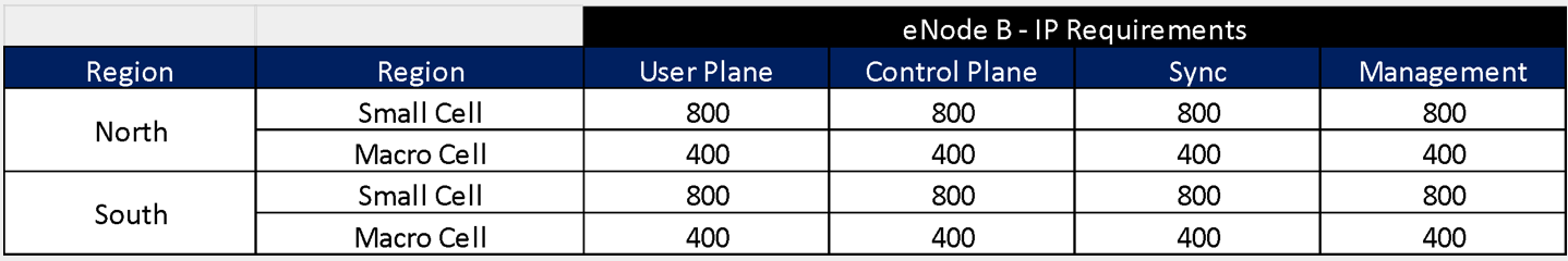
Table 23. IP Requirements for eNodeB Segment in Design Example
For the Router and MW O&M segments, no further subnetting is required. Table 24 displays the identified scenarios along with the total number of required IP addresses for each of these segments. The typical IP Ranges in Table 22 were used to calculate the total number of IP addresses.
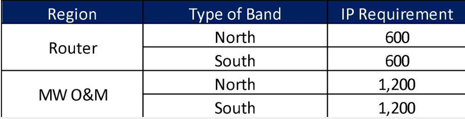
Table 24. IP Requirements for Router and MW O&M segments in Design Example
Step 3. IP Subnetting
Table 25 displays the Detailed IP Distribution Plan for the eNodeB segment obtained by applying the methodology in Section 3.3.
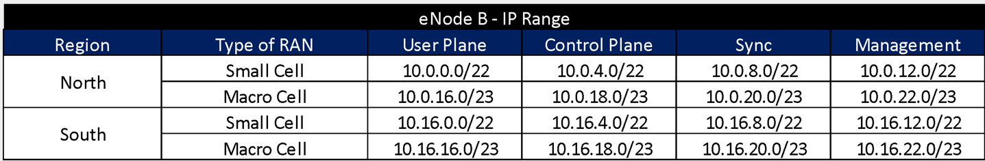
Table 25. Detailed IP Distribution Plan for eNodeB Segment in Design Example
Table 22 displays the Detailed IP Distribution Plan for the Router and MW O&M segments obtained by applying the methodology in Section 3.3.

Table 26. Detailed IP Distribution Plan for Router and MW O&M segments in Design Example
>
4.2.6 Site Tx Equipment Definition
To simplify the design process, the Site Tx Equipment Definition is performed based on the scenarios generated in the Tx Model Site Catalog. For each site, the transport site data is mapped to one of the scenarios in the Model Site Catalog.
Design Example
Table 27 displays the Tx Equipment Definition for the Design Example using the Model Sites defined in Table 11.
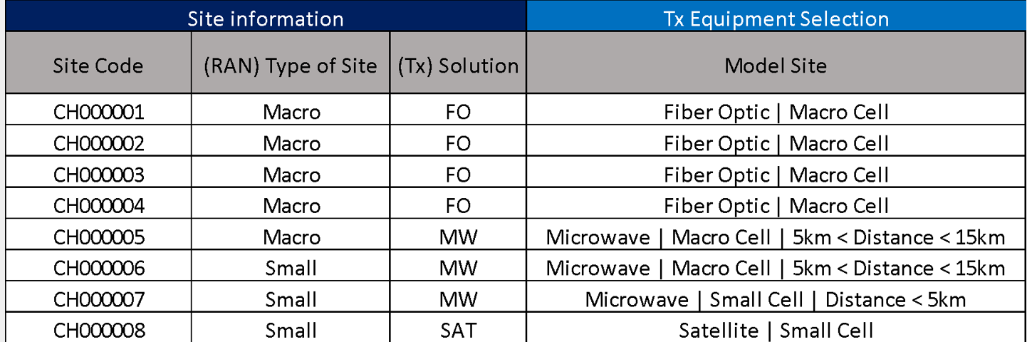
Table 27. Tx Equipment Definition for Design Example
>
4.2.7 Tx Network Resources Allocation
This section describes the methodology to perform the IP Address allocations tasks for LTE eNodeB planes and transport equipment and 4G services.
The IP addresses allocated to the network elements must be unique, this means that the same address must not be used for another element, even if the elements are in isolated areas.
IP Address Allocation
In the eNodeB, IP addresses need to be assigned for the user, control, management and synchronization plane. These elements must follow the Detailed IP Distribution Plan.
The IP address allocation process must be performed following the methodology presented in Section 3.4 and considering the typical IP Ranges presented in Table 22.
Tx Equipment Resources Allocation
Besides IP addresses, the transport equipment requires the following information to completely define the network resources:
Furthermore, in case a 3rd party is used, the following information is required:
Design Example
The allocation of the IP addresses for the eNodeB planes is done following the methodology presented in Section 3.3 using the Detailed IP Distribution Plan defined in Table 25. Table 28 displays the final IP address allocation for eNodeBs planes.
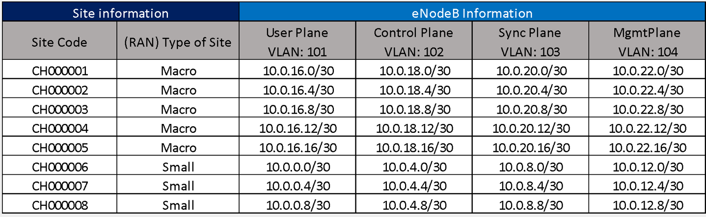
Table 28. eNodeB IP Address and VLAN Allocation for Design Example
All the /30 segments in Table 28 comply with the following definition. The segment 10.0.16.0/30 is taken as example for better explanation:
Similarly, Table 29 displays the IP address allocation for Routers & MW Radios.
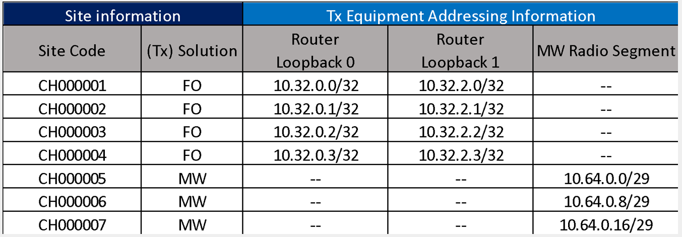
Table 29. Tx Equipment IP Address Allocation for Design Example
>
4.2.8 Tx Link Design
The Tx Link Design tasks for the available transport technologies must be performed following the methodologies presented in Section 3.
The level of automation implemented depends on the characteristics of the selected tools to perform the design tasks. Furthermore, the analysis can be done in batch mode or in a one by one fashion.
Finally, it is important to maintain a repository with the reports for all the transport links analyzed that can be accessed for all the team members, in particular, the deployment team.
4.2.8.1 Fiber Optic Link Design Guidelines
Table 30 displays the Fiber Optic Link Design Guidelines to be considered in the Link Design.
|
Characteristic |
Engineering Guideline |
|
Fiber Optic Interfaces |
– 1G interface per Last-mile Links |
|
– 10G interface per Aggregation Links |
|
|
*Capacity Safety Margin of 20% of interface capacity |
|
|
Length wave |
-1310 nm for 1000BASE-LSX |
|
Fiber Loss |
0.35 dB/km |
Table 30. Guidelines for Fiber Optic Link Design
>
4.2.8.2 Microwave Link Design Guidelines
Table 31 displays the Microwave Link Design Guidelines to be considered in the Link Design.
|
Characteristic |
Engineering Guideline |
|
Availability |
-Last-mile Link: 99,9% |
|
Frequency Band Selection |
– Unlicensed 5GHz for distances < 5km |
|
– Licensed 15GHz for distances in the range of 5km-15km |
|
|
– Licensed 7GHz for distances in the range of 10km-25km |
|
|
Microwave Link Capacity |
– 50Mbps – 100Mbps per Last-mile Links |
|
– 100Mbps – 250Mbps per Aggregation Links |
|
|
*Capacity Safety Margin of 20% of link capacity |
|
|
Terrain Database |
The terrain database must have a resolution of at least 500m. |
|
Rain Attenuation Calculation |
ITU method Recommendation ITU-R P.530-7 / 8 |
Table 31. Guidelines for Microwave Link Design
>
Design Example
Fiber Optic Link Design
The methodology presented in Section 3.1 is applied to generate the Fiber Optic Link Design following the guidelines in Table 30. The results are displayed in Table 32.
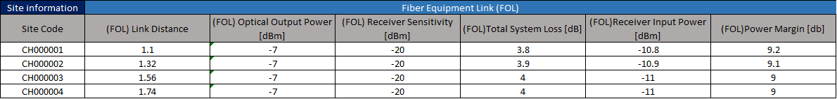
Table 32. Fiber Optic Link Designs for Design Example
Microwave Link Design
The methodology presented in Section 3.2 is applied to generate the Microwave Link Design following the guidelines in Table 31. Figure 20 displays the MW link profiles for Design Example.
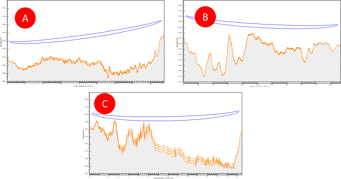
Figure 20. MW Link Profiles for Design Example
The results of the Link Budget are displayed in shown in Table 33.
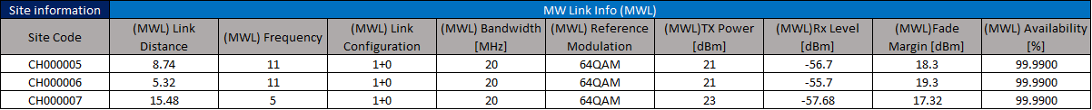
Table 33. Microwave Link Designs for Design Example
In addition, NaaS Operator can use the Tx LLD Report Template as a base to create their own version.
>
4.2.9 DF Generation
The Transport Datafill is a document that consolidates the required information to implement the transport solution in a site. The following subsections describe procedures to perform the Datafill Generation.
To simplify the overall process and standardize the Datafill generation, a Template that contains the consolidated transport information must be defined and adopted by the NaaS operator. It is highly recommended that the Datafill Template is divided in the following sections:
Furthermore, there are two main approaches to consolidate the Datafill Generation Process:
The recommended approach for small networks (e.g. 50 sites) is the Per-site Datafill approach. For more complex networks, the Per-Technology Datafill.
Design Example
For space considerations, the transport Datafill for the transport links in the Design Example are included as part of the Tx LLD Report Template.
>
4.2.10 BoM Generation
A bill of materials (also known as a BOM) is a comprehensive list of parts, items, assemblies and other materials required to implement the transport solution during the deployment phase. Following is a high level list of information to include into BOM record:
Following are key requirements that BoM management should address to optimize the process:
Design Example
The Bill of Materials that considers the equipment required for all the scenarios in the Design Example is displayed in Table 34.
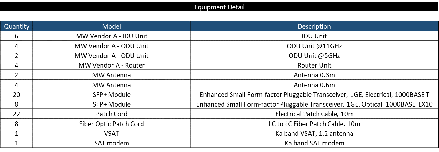
Table 34. Bill of Materials for the scenarios in Design Example
In addition, NaaS Operator can use the Tx LLD Report Template as a base to create their own version.
>
4.3 NaaS Operator End-to-End Process Definition
NaaS operators can use the generic process design as a base to develop its own version according to its limitations and constraints. In order to adapt the generic process a deeper analysis of the process can be performed.
Analyzing the provided generic process design, activities can be classified into two groups:
The approach presented on this section will focus on continuous activities as they consume the majority of the resources. Following some guidelines that NaaS operator should consider in order to customize its own process:
Finally, it is highly recommended that NaaS operators execute a Critical Path Analysis over its process version to further optimization.
5 LLD Recommendation
Methodology to consolidate and generate a final LLD recommendation.
5.1 LLD Recommendation Format & Structure
The main deliverable is the LLD Recommendation which contains the overall technical solution description and basic configuration parameters required to implement the Tx Transport network. The LLD Recommendation shall contain the following aspects that should be consolidated into a single location that is accessible by all the members of the team (e.g. an Excel Workbook in a shared repository):
5.2 LLD Recommendation Generation
Generation of the Reference Architecture following the format and structure established. NaaS Operator can use the Tx LLD Report Template as a reference to create their own version.
1. RAN Network HLD
A RAN High Level Design (HLD) is a critical engineering first step in expanding coverage into a new market, community, or area‒whether by deploying a brand new network for a greenfield project or by integrating a new radio access technology (RAT) on an existing network in an overlay initiative. It typically follows a business commitment to deploy but can also be used to inform the business case to establish or expand coverage.
Two scenarios can be identified: greenfield and overlay. The key characteristic of greenfield scenarios is the lack of existing infrastructure while in an overlay scenario there is a preexisting network. The greenfield scenario creates a higher CAPEX burden and focuses on reaching new market shares. On the other hand, the overlay scenario focuses on offering new services and improving end users quality of service (QoS) while leveraging existing infrastructure that implies a much lower CAPEX.
NaaS playbooks framework shown in Figure 1 displays the playbook modules and their relationship to the RAN HLD.
The Strategic Plan & Scope and High-Level Network Architecture modules provide the business and technical context for the NaaS operator and have direct impact and influence on many aspects of the network design.
This RAN HLD module is included within the network design area and has direct relation with TX backhaul HLD, backbone HLD, and mobile core HLD. The generated output of this module will serve as a required input for the RAN LLD module.
Figure 2 presents the RAN HLD functional view where the main functional components are exhibited. Critical module inputs are further described and examined in section 2.2. In addition, guidance and methodologies to execute the tasks included within each function are described in Section 3.
Figure 1 Network deployment and management framework
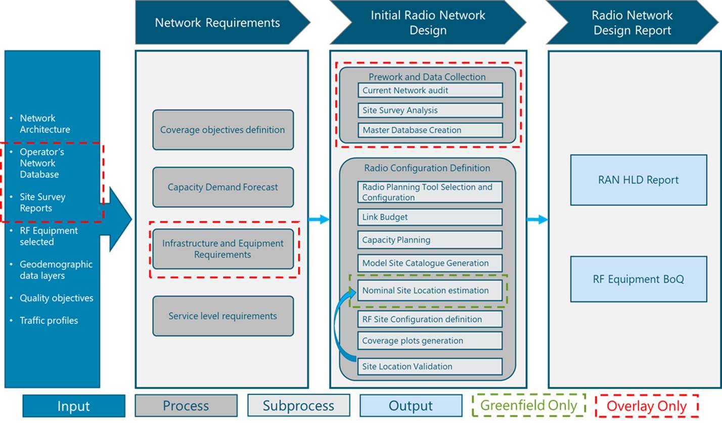
Figure 2 RAN HLD module functional view
2 HLD Fundamentals
This section presents a general overview of the baseline concepts to develop a RAN network design.
2.1 Radio Access Network Environment
A RAN design refers to the engineering process of integrating new mobile services on a previously uncovered area (greenfield scenario) or enhancing the existing ones on an already live network (overlay scenario). The RAN HLD process needs extensive RF dimensioning accompanied by iterations of radio planning (in the greenfield scenario for the selection of the final site locations).
The investment made for a deployment generally depends on the scope and radio technology of the design. Cellular base stations and RF equipment are expensive long-term investments for the operator and, as such, any operator will prefer to deploy the minimum number of sites to provide the optimal required coverage. The ideal site maximizes coverage in the intended area while minimizing interference.
Accurate design minimizes the need to add additional sites or relocate existing ones to meet the coverage and capacity needs.
2.2 Radio Access Network Design Inputs Description
Table 1 presents a description of module input data and candidate sources required for a RAN HLD. Furthermore, the impact of each input on the design process is examined.
|
Input Required |
Description |
Impact |
Source |
|
Network Architecture |
High level view of the overall network |
Will help to define the required site configuration |
High Level Network Architecture Module |
|
Operators Network Database* |
Information regarding deployed network (e.g., physical site configuration and location, number of sectors and cells per site, and site and cell logical identifiers) |
An updated database will clearly display each sites characteristics that will boost the overlay design |
Operator Network Data |
|
Site Survey Reports* |
Reports of inspections of physical sites to gather relevant information (e.g. equipment inventory, photographic documentation) |
Will significantly reduce rework when any difference is present between operators network database and physical installation |
Site Survey Module |
|
RF Equipment Generic Specifications |
Specifications of the RF equipment regarding frequency, channel bandwidth and capacity |
Accurate configuration for radio planning |
High Level Network Architecture Module |
|
Geodemographic Data Layers |
Digital terrain maps with geographic information: ●Clutter ●Terrain ●Population distribution maps |
Accurate dimensioning |
Operator Network Data |
|
Quality Objectives |
Provides QoS requirements to be met in the network dimensioning exercise |
Define coverage dimensioning |
Engineering Specifications Module |
|
Traffic Model* |
Summary of the number of subscribers in the network, their demanded services and subscriber usage level. |
Define capacity dimensioning |
Operator Network Data |
|
* Inputs required only for Overlay RAN initiatives |
|||
Table 1 Module input data
2.3 Coverage Dimensioning
The objective of coverage dimensioning is to find the minimum number of sites to achieve the required coverage and establish the coverage area provided by each site. Coverage area refers to the area where the energy radiated by the base station can be received by the end users equipment (UE) with an acceptable level and determines the maximum area that can be covered by a base station.
A dimensioning exercise gives an estimate that is then used for detailed planning of the network.
Various factors must be considered during network coverage dimensioning and setting of these parameters will affect coverage radius and the quantity of base stations. Factors such as the propagation environment and equipment characteristics will influence overall coverage dimensioning. Deeper insights into the coverage dimensioning process will be given in sections 3.4 and 3.5.
2.4 Capacity Dimensioning
Capacity dimensioning is used to determine the maximum data throughput and number of simultaneous users supported by a single cell and eventually the required number of base stations to meet the traffic demands in the desired area.
System capacity can be defined as the maximum aggregated data rate supported while meeting quality of service targets. The greater a sites capacity, the higher amount of data is supported, and more mobile subscribers can be connected to that base station at a given time, thereby reducing the amount of base stations that are required. This reduction would lead to capital and operational efficiencies for the network operator.
The technical aspects of coverage dimensioning are discussed in Primer on Dimensioning Principles.
2.5 Site Evaluation
Site evaluation is the process performed to select the final location to deploy a new base station based on the site survey result and transport solution criteria. Figure 3 displays a graphical summary of the site evaluation criteria points that are explained below.
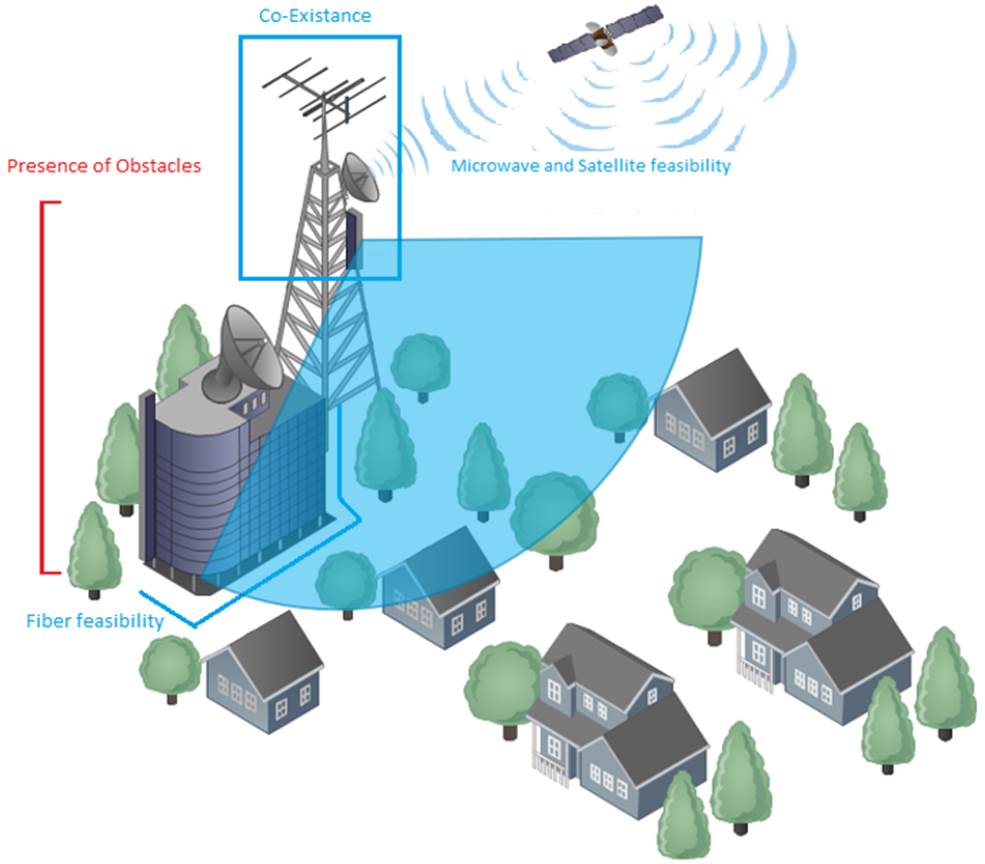
Figure 3 Site evaluation criteria point
a) Presence of obstacles:
Obstacles such as foliage or buildings that could attenuate the antenna beam must be clearly identified as this will represent a major coverage degradation. Upcoming obstructions, such as new buildings planned or under construction should also be considered.
As far as possible, the path between the antenna and the area to be covered should be clear of man-made obstructions and foliage.
b) Height evaluation
Height of a proposed new site (nominal site) is an important parameter as it directly impacts its coverage. Site height must be compared with the surrounding environment (buildings, trees, and any other possible obstruction). Natural high-elevation locations (such as hills) can be leveraged for the installation of new sites to get better coverage compared with floor level installations. By placing the transmitter on a high tower or leveraging terrain elevation, the transmitter will be able to achieve a greater coverage than by placing it on lower heights. The higher the transmitter is from the floor, the following mechanisms are improved:
c) Co-existence
Radio transmitters near the location candidate or at the same site location can add interference levels to the new site that will impact service quality of the new cell. Interference can be caused by any electric equipment operating near the base station (even if operating on different frequencies) as equipment can introduce spurious harmonics that translate in the degradation of the desired signal. Major sources of interference are usually other base stations operating at different frequencies and power equipment.
Acceptable interference levels can be taken based on equipment specifications. However, measuring interference levels can be impractical. A rule of thumb for LTE deployments is that the system requires 40 dB of isolation. If the antennas have a vertical separation, there should be at least 0.2 m between the base of one antenna and the top of the other antenna. If antennas have a horizontal physical separation and a beamwidth of 65, there should be at least 0.5 m between them. These separations are shown in Figure 4.
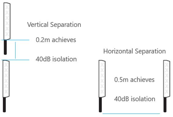
Figure 4 Vertical and horizontal separation to achieve isolation
d) Feasibility for backhaul solution deployment
The transport team will need to validate the site location according to transport solution criteria. Criteria will depend on the transport solution selected for the site. Transport solutions and their corresponding criteria are briefly summarized in Table 2.
|
Feasibility Criteria |
|
|
Fiber Optic |
Available path/road for the deployment of the fiber |
|
Microwave |
LOS between the site and a transport node |
|
Satellite |
Base station within the satellite footprint |
Table 2 Feasibility criteria for backhaul solutions
If the site location doesnt comply with such criteria, it must be relocated.
Site selection may also consider other non-RF related criteria such as availability of power supply and space for equipment. These points will be covered in the Deployment module.
3 Functions & Methodologies
Methodologies to perform critical tasks/subtasks involved in the RAN design process.
3.1 Current Network Audit (Overlay Design)
This section applies only for overlay projects, the user interested in greenfield only, can skip directly to Section 3.3. In overlay RAN projects, the NaaS operator will deploy a new RAT on top of its current network. To have a feasible source of information about the existing RATs and the new one, an audit of the current network is required. The audit process comprises data collection from the OSS tools and from operators database/inventory. Information gathered from these two sources will be consolidated into one single document that will present the current state of the overall RAN. The process is detailed in the following sections.
3.1.1 Operations Support Systems Tools Data Collection
RAN vendors implement OSS tools, through them NaaS operators monitor and manage their network (e.g., Ericssons OSS Common Explorer, Huaweis U2000, Nokias NetAct). OSS tools provide data from the live network and must be considered as the most reliable source to identify the status (on-air, off-air) and logical configuration of each site in the network.
Furthermore, OSS tools are the vehicle to obtain the information required in the audit process: Site and cell names, site and cell logical identifiers per RAT such as physical cell identity (PCI) for LTE, primary scrambling code (PSC) for 3G and base station identity code (BSIC) for 2G. With this information, designers can determine the number of sectors and carriers per RAT of each sitethe first step in the candidate selection. The basic principle of a network audit process is to collect all the available OSS networks information. Table 3 and Table 4 display the network information required for the network audit. These parameters are necessary to identify each site and its RF configuration. Its important to notice that some identifier names can vary from vendor to vendor.
|
Basic Site and Cell Name per Technology |
||
|
LTE |
WCDMA |
GSM |
|
Site Name Site Code eNodeB Code Cell Name Cell Code Site status Cell status |
Site Name Site Code Cell Name Cell Code Cell Name Site status Cell status |
Site Name Site Code Cell Name Cell Code TRX Name TRX Code Site status Cell status |
Table 3 Site and cell names
|
Basic Logical Site and Cell Identifiers per Technology |
||
|
LTE |
WCDMA |
GSM |
|
PCI PRACH Bandwidth TAC RAC EARFCN MME Code |
PSC UARFC (UTRA Absolute Radio Frequency Channel Number) URA LAC RAC SAC RNC Name RNC Code |
BSC Name BSC Code BSIC (NCC+BCC) TRX No. BCCH HSS LAC RAC |
Table 4 Site and cell logical identifiers
In addition, some physical site configuration such as azimuth, latitude and longitude can be collected from the OSS tool (depends on each vendor tools limitations). Nevertheless, Site Survey report is the most accurate source to obtain physical information (as will be described in section 3.2). Table 5 displays required physical information.
|
Basic Physical Site Parameters for All technologies. |
|
Type of Site Frequency Band Latitude & Longitude Ground Height Antenna Tilt (Electrical +Mechanical) |
Table 5 Physical site parameters
OSS tools allow NaaS operators to export the network data in different formats. The default choice is to extract network information in Excel spreadsheets. Exportable information makes data analysis and collection easier for NaaS operators.
The source of the data varies based on the technology: In GSM-2G and UMTS-3G, RAN information sources are network controllers (base station controller for 2G and radio network controller for 3G) while for LTE-4G sources are base stations themselves; they can be organized in groups defined by the operator (e.g., by region, by MME). Network designers must download information from the whole network.
All network information collected should be unified in one file, preferably in an Excel format, one sheet or workbook per RAT. An Excel file enables NaaS operator to manage, update and filter information easily.
3.1.2 Naas Operators Network Database Analysis
Besides OSS information, NaaS operators have their own network database that is the as-built database for all physical configurations. Frequently, an operators database is out of date mainly because some network changes arent always reflected in it. Nevertheless, this database is always relied on for physical site configuration coming from previous RAT deployments. Physical information to be obtained from operators database is: longitude, latitude, azimuth, electrical tilt, mechanical tilt, and antenna or tower height.
If the NaaS operators have more than one network database, its necessary to consolidate the information in one. The consolidation process is composed by three steps:
Its important to clarify that the process must be applied per RAT since the objective is built to a database with the physical configuration per technology of each site in the network.
3.1.3 OSS Information and Operators Database Consolidation
To finalize the current network audit, the information collected from the OSS tools (site and cell names, logical identifiers) should be complemented with the consolidated operators database. (site physical configuration).
Since the OSS information is the most accurate source of data, sites and sectors contained in the consolidated database that dont appear in the OSS tools should be removed; NaaS operators must define the action points to clarify their status.
If there are sites and sectors from OSS tools missing in the consolidated database, NaaS operators should evaluate the possibility to do a site survey.
The physical site configuration obtained through OSS tools should be compared with the consolidated database; the Naas operator must evaluate its relevance. Physical information from OSS tools could be not updated or be accurate since theyre mainly used to manage logical configuration in contrast with consolidated database that comes from site surveys made in previous RAT deployments.
The information should be on a single point of consultation. This point can go from a web-shared spreadsheet (Google Sheet, Office365) to an inventory management solution. Table 6 shows a summary of some open source inventory management tools.
|
Feature |
Kuwaiba |
AssetTiger |
ManageEngine AssetExplorer |
Snipe-IT |
|
Upgrade Cost |
Free |
$100/year |
$955/year |
$399.9/year |
|
Free Usage Limit |
Unlimited objects and users |
N/A |
N/A |
N/A |
|
Mobile App |
No |
Yes |
Yes |
Yes |
Table 6 Inventory management tools
A NaaS operator can use the Network Information Management and Inventory for the creation of its consolidated database.
3.2 Site Survey Analysis (Overlay Design)
The current network audit (section 3.1) focuses on consolidating information available in existing databases (OSS tools and operators database). However, regarding physical information, the most reliable source of information is existing site survey reports. An SSR contains extensive physical information about the sites in the network. During the HLD phase for overlay scenarios, NaaS operators should be focused on information regarding geographical site position, physical configuration, and hardware installed.
During the analysis of SSRs, designers must validate or update physical site configuration defined in the database created after the current network audit. The final audit database must be aligned with SSR information.
By extracting information about installed RF equipment per site, NaaS operators can identify candidate site configurations. This information will be useful to define the standard configurations.
Through the SSR analysis, RF hardware already installed is examined to evaluate the necessity to update the existing equipment or reuse it (that may reduce the deployment investment). Installed equipment can be reused if it has enough capacity and/or equipment capabilities (radio units and antennas operating band) to support the new overlay technology
Under the scope of an overlay RAN HLD, reusable hardware can be composed of antennas, radio units (RRUs), and baseband units (BBUs). More details are in section 4.2.4
3.3 Master Database Creation
The master database consolidates information obtained from the current network audit and site survey analysis and must be the source of truth for network information containing information from all sites in the network. Collection of the information in only one source is the Master Databases objective. furthermore, its essential to obtain accurate coverage plots and one of the main inputs for the deployment phase.
The master database creation process is divided in three steps:
- Network Current Audit Consolidation between OSS tools information (logical site configuration) and operators database (physical configuration) to generate final audit database.
- Site Survey Analysis Since the SSRs contain the most accurate physical site configuration, the final audit database must be updated with the available reports.
- Site Categorization All sites in the network must be categorized as candidate or non-candidate and each candidate must be associated with one standard configuration (section 3.9). An existing site can be considered as a candidate if it complies with basic criteria such as: available tower space, available power supply, and acceptable rental costs, among others. A NaaS operator can use the Site Location Validation Questionnaire template to evaluate a site as a candidate or non-candidate.
Basic information to be contained in the master database is:
Note: Site category can be defined based on the Site Location Validation Questionnaire template
For greenfield projects, a master database or inventory is to be created as well to keep track of the designs and register sites on-air as deployment progresses.
NaaS Operator can make use of the Master Database Template to work on its own version or use one of the Inventory Tools described in section 3.2.
3.4 Link Budget
Radio link budget (RLB) is the first step to estimate the required number of sites to cover a certain area. RLB computes the power received by the user equipment (UE) given a specific transmit power from the base station.
Received power is obtained by adding transmit power to both base stations and UEs antenna gains and subtracting feeder losses, path loss, body loss, shadowing and interference margins. Eq 1 summarizes the RLB process. Figure 5 displays a representation of the RBL process in a mobile system.
![]()
(Eq. 1)
Where:
● ![]() – Received Power
– Received Power
● ![]() – Transmitter Power
– Transmitter Power
● ![]() – Gain of the base station antenna
– Gain of the base station antenna
● ![]() – Gain of the User Equipment antenna
– Gain of the User Equipment antenna
● ![]() – Feeder Loss
– Feeder Loss
Indicates the signal loss caused by various devices (e.g., jumpers, cables) located in the path from the transmitter to the antenna
● ![]() – Path Loss
– Path Loss
● ![]() – Body Loss
– Body Loss
Indicates loss generated due to signal blocking and absorption when the user’s equipment is close to the person’s body.
● ![]() – Shadow Margin
– Shadow Margin
An extra “loss” is considered to account for obstacle absorption of the radio signal.
● ![]() – Interference Margin
– Interference Margin
An extra “loss” is considered to account for degradation in the received signal due to interference from other base stations.
Figure 5. Radio Link Budget representation.
Eq. 1 must be rearranged to perform coverage dimensioning using RBL. UE received power can be substituted with its sensitivity (minimum required power for the signal to be decoded at the UE). Considering this, the designer will be able to estimate the maximum loss that the signal can suffer for the UE to work properly. As the main loss present in the mobile system is due to the path loss, a maximum allowed path loss (MAPL) can be estimated as shown in Eq. 2:
![]()
(Eq. 2)
Where:
● ![]() – Sensitivity of the user equipment
– Sensitivity of the user equipment
Once the MAPL is known, the cell radius can be obtained using a propagation model. Propagation models are used to estimate the attenuation of the radio wave as it traverses its path. A variety of propagation models exist, and their application is determined by two main factors:
- Operating frequency.
- Morphology (clutter) under consideration. Clutters can be classified as follows:
- Urban This environment consists mainly of large buildings (that produce major attenuation) and small density of foliage.
- Suburban This environment presents wide-ranging housing areas that includes some vegetation. Suburban environments are mostly found at the border of urban areas, spreading outward from the city centers.
- Rural This environment represents wide areas with a small density of buildings and large density of foliage. Major attenuation is due to the foliage present on the terrain.
The designer can follow these criteria to quickly choose a propagation model:
The technical aspects of propagation models are discussed in the Primer on Propagation Models..
Okumura-Hata and COST-231 models require the height of the base station as an input for the loss prediction. Network designers must consider the fact that the selection of a transmitters height represents a trade-off between coverage, number of sites, and financial investment.
Higher base stations represent better coverage per site, requiring fewer sites per region. However, higher sites cost more to build and cost goes up exponentially with tower height. Network designers must find a balance between the number of sites per region and the financial constraints involving site height. Further guidance and a design example are provided in section 4.2.8.
If path loss is known (shown in Eq. 2), then cell radius can be computed by solving the propagation models equation for d (see Primer); this can be done practically using the Widget for Coverage-Based Site Count.
Table 7 shows examples for 700MHz and 1800MHz:
|
Frequency |
Transmitter Height |
Transmit Power |
Cell Radius |
|
700 MHz |
15 m |
20 W |
4.70 Km |
|
30 W |
5.24 Km |
||
|
700 MHz |
20 m |
20 W |
5.43 Km |
|
30 W |
6.07 Km |
||
|
700 MHz |
30 m |
20 W |
6.73 Km |
|
30 W |
7.55 Km |
||
|
1800 MHz |
15 m |
20 W |
0.84 Km |
|
30 W |
0.94 Km |
||
|
1800 MHz |
20 m |
20 W |
0.94 Km |
|
30 W |
1.05 Km |
||
|
1800 MHz |
30 m |
20 W |
1.10 Km |
|
30 W |
1.23 Km |
Table 7 Cell radius calculation
Cell radius based on link budget should be taken as the best case as its based on average calculations and doesnt take into account all obstacles and propagation mechanisms of the signal.
3.5 Coverage-Based Site Count
Once cell radius is estimated, it can be used to calculate the number of sites required to cover the whole area with respect to the cell radius d. By convention, cell coverage area is assumed to be hexagonal as shown in Figure 6.
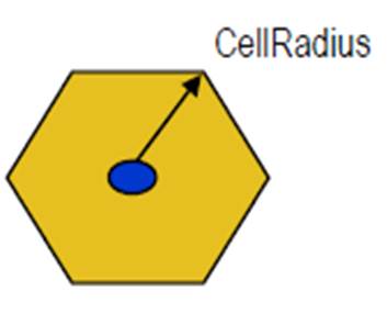
Figure 6 Coverage area of a radio site
For a hexagonal site, coverage area can be calculated as follows:
![]()
(Eq. 3)
The number of sites to be deployed can be calculated from the coverage area and the required area to be covered (deployment area) as follows:
![]()
(Eq. 4)
Even the link budget is based entirely on mathematical equations; a complete RAN HLD can be achieved by only applying it. A more detailed planning can be done by using a radio planning tool (RPT) thanks to the use of terrain information. However, the use of an RPT is optional in uncovered rural environments.
A NaaS operator can use the Widget for Coverage-Based Site Count for this task.
3.6 Radio Planning Tool Selection
When a RAN design project is to be performed, RPTs can be used for simulations and location of new sites. These make use of sophisticated and detailed terrain maps: terrain elevation maps, demographic distribution maps, and clutters that make the design more detailed. Thanks to this, RPTs can use several more complex propagation models that account the terrains profile (e.g., mountains) into the loss prediction (details about RPT configuration are out of the scope of this module).
However, the use of an RPT in the RAN HLD is optional for uncovered rural areas. As will be shown later, location of new sites and coverage planning can be done following the link budget procedure.
There is a wide variety of RPTs that can be classified in several manners: licensed and unlicensed, carrier and WISP grade, and web-based. To simplify RPT selection, Table 8 displays a summarized description of some RPTs.
Table 8 Summary of radio planning tools
A first step in selecting an RPT is to always consider the budget of the operator.
The next step is to define which tool features will be required. For the creation of the RAN HLD, at a minimum a designer needs to be able to estimate the transmitter height, transmitter power, number of sites, and sectors per siteas well as be able to locate the site in the desired location (described in section 3.10). Site planning will be a desired feature to speed the HLD process but not a mandatory one. Additional features such as frequency planning, neighbor planning, physical optimization, and database management will impact the low-level design (LLD). An operator can selecting an RPT just for the HLD process, which translates in selecting a WISP grade tool.
Table 9 summarizes features of the tools listed above. An operator can choose an appropriate RPT based on it.
|
|
|
Carrier Grade Tools |
WISP Grade Tools |
||
|
Planning Tool |
Atoll |
Mentum Planet |
Radio Mobile |
Xirio Online Planning Tool |
|
|
Estimation of Sites Azimuth & Tilts |
Yes |
Yes |
Yes |
Yes |
|
|
Support for Detailed Map information |
Yes |
Yes |
Yes |
Yes |
|
|
Site Planning |
Yes |
Yes |
Yes |
Yes |
|
|
Frequency Planning |
Yes |
Yes |
No |
Yes |
|
|
Neighbor Planning |
Yes |
Yes |
No |
No |
|
|
Physical Optimization |
Yes |
Yes |
No |
No |
|
|
Database Management |
Yes |
Yes |
No |
No |
|
|
Price |
High |
High |
Free |
Medium |
|
Table 9 Summary of radio planning tools and features
3.7 Capacity Based Dimensioning
Radio equipment has capacity limitations driven by two main factors:
- The maximum number of simultaneous active users that a single base station can serve.
- The maximum throughput supported.
These two factors must be analyzed separately and their results compared to compute the required number of radio units based on capacity requirements.
3.7.1 User-Based Capacity Dimensioning
This is defined as the maximum number of simultaneous active users varies from one equipment to another. To have the exact value, network designers must identify it from the product description of the specific equipment. However, a good approximation is to consider that 100 simultaneous active users are supported per radio equipment. The following steps must be followed for the user-based capacity dimensioning.
Subscriber Forecast:
Network designers must obtain the total number of subscribers that will be served in the required area. This value is calculated by the following equation:
![]()
(Eq. 5)
Where
-
 – Population Target: Reflects the total number of inhabitants in the area. This quantity exclusively depends on the target area defined by the NaaS operator.
  – Service Penetration: Percentage of the overall population that will be covered. This quantity is based on the NaaS operators business case. Values between 40% and 60% are commonly used for rural environments with no competition.
Active Users Forecast
Not all subscribers will always be served simultaneously. The percentage of active users in the busy hour (the time where a peak in the service exists) is considered to dimension the number of active users in a network.
![]()
(Eq. 6)
Where
-
 Is the percentage of subscribers who are active in the busy hour of the day. This input can be Provided by the NaaS operator. However, 5% can be taken as a starting value.
Equipment Dimensioning
Finally, the number of active users must be compared with the maximum active users supported by the radio equipment.
![]()
(Eq. 7)
Where
 Is the maximum concurrent users per eNB.
3.7.2 Throughput-Based Capacity Dimensioning
In a similar way that the base station supports a determined number of simultaneous active users, it also has a limited downlink (DL) and uplink (UL) throughput. For this reason, an evaluation of the overall DL and UL throughput must be done to evaluate the required number of sites.
The first step is to compute the overall DL and UL traffic that will be generated by the active subscribers during the busy hour (time frame of one day where the maximum amount of traffic is carried in the network.). Eq.8 and Eq.9 show how to compute these figures for DL and UL respectively.
![]()
(Eq. 8)
![]()
(Eq. 9)
Where:
-
 &
&  – Average DL & UL throughput that the network carries during the busiest hour of the day. Depending on the specific environment, typical values go from 16 kbps to 128 kbps.
 -
 (Peak-to-Average Ratio) Is the relation between the peak throughput and the average throughput. As bursty traffic is common, values between 6 and 10 can be used if no previous data is available.
 -
 (Overprovisioning Factor) Is a percentage of the total eNB capacity that will be used for the dimensioning, leaving the rest percentage of the capacity as a backup for special events or future network expansion. Typical values are between 70% and 90%.
 - Is the relation between maximum throughput and subscriber throughput in the busy hour.
The next step is to compare the calculated DL and UL traffic with radio equipments average throughput capacity as shown in Eq. 10 and Eq. 11. If equipment average throughput data is not available, the typical values of an LTE system can be considered. Table 10 displays cell average throughput for different scenarios and bandwidths.
|
5 |
8 |
5 |
|
10 |
17 |
10 |
|
15 |
25 |
15 |
|
20 |
33 |
20 |
Table 10 Typical average sector throughput for LTE-FDD (considering MIMO 2×2)
The comparison between overall DL and UL throughput and equipment average throughput capacity will result in the required number of radio equipment to support the DL and UL demand.
![]()
(Eq. 10)
![]()
(Eq. 11)
Where:
-
 &
&  eNodeBs average DL and UL throughput
 -
 &
&  Maximum allowed DL and UL rate per subscriber.
The required number of eNodeBs is calculated as the maximum between ![]() and
and ![]() :
:
![]()
(Eq. 12)
3.7.3 RAN Equipment Count
Final eNodeB count will be obtained from the comparison of the user-based vs. the throughput-based capacity dimensioning. The maximum between ![]() and
and ![]() will give as result the final eNodeB count.
will give as result the final eNodeB count.
![]()
(Eq. 13)
This calculation can be easily done through the Widget for Capacity-Based Site Count.
3.8 Standard Configurations Definition
High-level site configuration is a combination of the following parameters: operating frequency, antenna height, transmitter power, number of sectors, and type of antenna. Based on the combination of these parameters, network designers can create specific configurations, simulate them and finally select that one performs better in terms of coverage, site count and cost. Deeper insight into the selection of the best configuration is made in section 4.2.8.
Based on RF specifications from RAN architecture module, standard configurations must be defined and registered.
The following are the steps to define standard configurations:
- Various combinations of antenna height, transmitter power and number of sectors should be considered. At least one macro cell and one small cell configuration should be considered based on Table 11 below.
- For each combination, cell radius can be calculated and a quick dimensioning to obtain the number of sites can be performed as indicated in section 3.5.
- Based on cell radius and feasible options regarding tower height and transmit power, select standard configurations to be used for nominal site location estimation.
|
Base Station Type |
Antenna Height |
# of Sectors |
Transmitter Power |
|
Macro Cell |
> 10m |
1 to 3 |
>10W |
|
Small Cell |
< 10m |
1 |
< 10W |
Table 11. Base Station categorization.
|
Cfg. ID |
Base Station Type |
Cell Bandwidth |
Operating Frequency |
Antenna Height |
# of Sectors |
Tx Power |
Cell Radius (Km) |
|
Config. 1 |
|
|
|
|
|
|
|
|
Config. 2 |
|
|
|
|
|
|
|
|
|
|
|
|
|
|
|
|
|
Config. n |
|
|
|
|
|
|
|
Table 12. Sites Configuration.
3.9 Nominal Site Location Estimation
After computing the number of base stations to cover the target area, the initial locations for those sites (referred to as nominal sites) must be defined. In a greenfield scenario, network designer must follow these next steps to establish the nominal site locations:
- Introduce third-party infrastructure locations (e.g., existing towers) to a GIS tool (e.g., Google Earth) as shown in Figure 7. The set of third-party infrastructures is an input to the network designer. If no third-party infrastructure is available, go to step 3.
- Create a hexagonal polygon, considering the location of existing towers as the hexagons center, as shown in Figure 8. The radius of the hexagon must be set using the Widget Coverage-Based Site Count using the height of the existing tower. Its a convention to consider the sites coverage area as having a hexagonal shape (when the real coverage region can have an irregular form). This is made to facilitate the filling of the coverage.
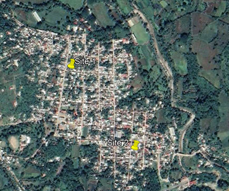
Figure 7. Location of existing infrastructure on the map.
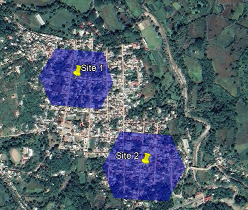
Figure 8. Hexagonal coverage for existing infrastructure.
- Uncovered areas of the desired region must be filled with hexagonal shapes until the whole region is covered. The center of each new hexagon will be considered as the sites location. Figure 9 displays this process.
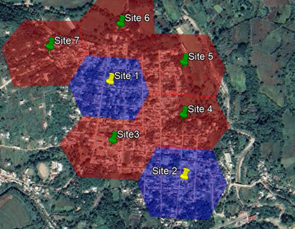
Figure 9 Filling of the remaining area
- The designer must verify that the sites defined in step 3 are located in valid locations:
Further discussion about valid and non-valid locations must be taken by NaaS operators
strategy team.
The network designer must notice that nominal locations can be changed due to external RF factors such as: transport solution feasibility, countrys regulations, or any point considered in the site evaluation criteria.
3.10 RF Site Configuration Definition
RF site configuration refers to the physical parameters in a radio base station: base station type, antenna height, number of sectors, and transmitting power. Standard configurations were previously defined in section 3.9.
Based on the site count (coverage and capacity), standard configurations, and nominal locations, the network designer is able to select the standard configuration(s) that best suit the coverage and capacity requirement.
Table 13 can help the designer to summarize site configurations.
|
Cfg. ID |
Number of Sites |
|
Cfg. 1 |
1 Site |
|
Cfg. 2 |
2 Sites |
|
|
|
|
Cfg. n |
n Sites |
Table 13. RF Sites Configuration distribution.
This represents an iterative process where several configurations must be analyzed to define which sites maximize the coverage region with the smaller number of base stations while keeping the CAPEX low. Implementation considerations are analyzed in section 4.2.8.
3.11 Site Location Validation
Once that nominal site locations have been estimated, location feasibility must be validated.
This can be done through satellite imagery or using existing information from the site; however,
in most cases a site survey must be performed.
The Site Location Validation Questionnaire is provided to the NaaS operator to evaluate all sites and candidate sites based on points previously discussed in section 2.5. Clauses in the questionnaire are considered as critical points. Thus, if a clause is not compliant, the site must be relocated or the candidate site dismissed.
Further guidance to perform site survey can be found in the Site Survey Module of the Playbook.
4E2E Process Flow
Generic yet customizable E2E process flowto perform the radio access design for the RAN. Through this section, a designexample for a greenfield scenario will be shown to display the application ofeach step of the E2E process.
4.1E2E ProcessOverview
Figure 10 displays ageneric E2E process to perform a greenfield RAN HLD. In addition, Figure 11displays the generic E2E process for an overlay RAN HLD.
For the greenfield scenario, locations tobe considered in the dimensioning process are initially defined in the CoverageObjectives Definition section. Service level requirement establishesradio access parameters that must be experienced by end users. Once the servicerequirements are established, a capacity demand forecast is performed to estimatetraffic growth in the future. The coverage and capacity dimensioning processpresents a methodology to compute the number of required sites based on bothcoverage and capacity constraints.
Standard radio configurations standardizeall possible radio base stations configurations to be used. RF configurationguides the designer into the selection of an optional radio planning tool; itis also a guidance for the selection of an optimal RF configuration and theestablishment of the adequate nominal site locations for radio sites. Site locationvalidation presents a methodology for the selection of the finallocations of the radio sites based on site evaluation criteria and transportsolution feasibility. Then a RF equipment BOQ determines the required equipmentto implement the RAN.
Figure 10 Greenfield RAN generic E2Eprocess description
In the case of an overlay scenario, someactivities are added due to the fact that this scenario considers an upgrade toan existing RAN. A coverage objectives definition and service levelrequirements are also defined in the overlay. However, this scenariorequires an infrastructure and equipment requirements analysis toidentify that equipment will be kept and that one should be changed for a newone. Also, a prework and data collection step is required to have anupdated view of the current network. Standard radio configurations arealso required to the new configurations. The candidate site definition processis analogous to the site location validation for greenfield, in that theexisting sites are assessed to define which ones will be upgraded with a newRAT. The remainder of activities will be the same, ending in an RF equipment BOQ.
Figure 11 Overlay RAN generic E2E process description
4.2Step-by-StepAnalysis
4.2.1Coverage ObjectivesDefinition
Analyzing and understanding coveragerequirements is the first step for the design process. Its essential to have awell-defined area to be covered. General requirements for the deployment of aRAN will generally be concerned with cost and time to market, so it can beinfluenced by the NaaS operators business strategy or predefined agreementswith MNOs. A simple process to define coverage objectives is described below:
- Identify the area to be covered Search for geographic areas with no 4G coverage, as uncovered areas will represent higher revenue opportunities.
- Identify Special locations Some special locations should be considered to have mandatory coverage (e.g., schools, hospitals, government buildings). Any location with strategic importance for the NaaS operator should be considered a special location.
- Identify covered population distribution How people are distributed in the selected area must be addressed to define that specific portion of the overall region.
DesignExample
In our example,the coverage objectives shown in Figure 12 have been defined by drawing apolygon in Google Earth and identifying populated areas in a rural town. Inaddition, two special locations are definedthe town hall and aschool.
Using Google Earth,the total area of the target polygon was calculated having as a result 0.8km2.
Population information wasobtained from census data ‒ 3683 total inhabitants.
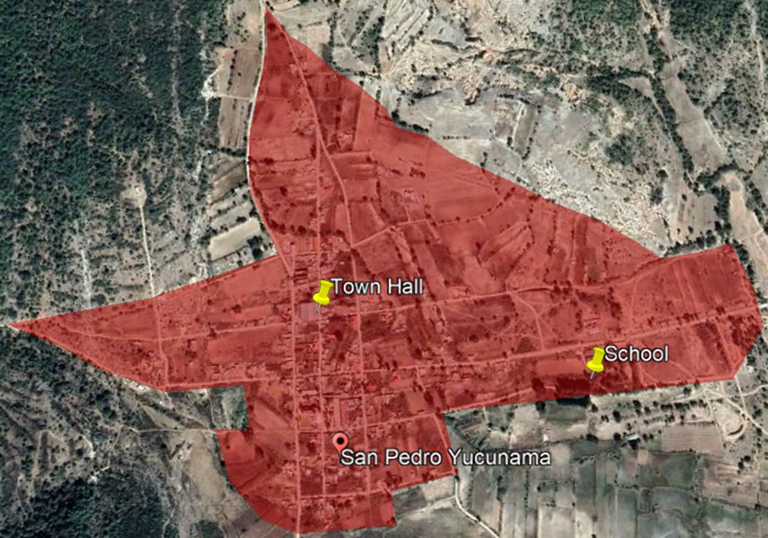
Figure 12 Coverage objective definition example
Dependencieswith other tasks
Service level requirementspresent the following dependencies:
Prerequisites
Outputs
4.2.2Service LevelRequirements
Mobile networks will support a variety ofsubscriber services. Some may be a key differentiating factor in the operatorsservice offering. Hence, the operator must define service level requirements interms of downlink (DL) and uplink (UL) throughput. Table 14 shows typicalservice requirements that can be considered by the NaaS operator.
|
Service Level |
Service Throughput (DL/UL) |
|
(Mbps) |
|
|
Service level A |
6 / 1.5 |
|
Service level B |
4 / 1 |
|
Service level C |
2 / 0.5 |
Table 14. Service Requirements Definition Example.
The NaaS operator can use the Widget for Capacity-based Site Count to evaluate theimpact on the number of sites for different t service level requirements.
Design Example
For the example case, we will consider servicelevel B for the capacity demand forecast estimation: DL throughput: 4 Mbps, ULthroughput: 1 Mbps.
Dependencies withother tasks
The definition of service levelrequirements is related with other tasks as detailed below.:
Outputs
4.2.3Capacity DemandForecast
Traffic forecast plays a major role incellular planning as its results must be considered for the dimensioning of thenetwork to overcome future capacity growth.
First, capacity at year 0 is estimatedusing one of two approaches:
- Apply the capacity dimensioning methodology shown in 3.8.
- For overlay initiatives, it can be taken from the sites current capacity.
Then capacity isforecasted based on a growth percentage per unit of time. Eq. 14 displays a formula for the estimation of a capacityforecast.
![]()
(Eq. 14)
Where n represents a planning horizon in thefuture and x is the growing factor. Initial capacity is considered asthe network overall number of users and DL and UL throughput.
Considering n as years is aconventional time frame for most calculations. Considering it as months willrepresent a very aggressive and unpractical consideration.
Standard values for x can be takenfrom 10% to 15%. Selection of a capacity growing factor will depend on how muchthe NaaS operator is expecting a growth on its network demand. However, aconservative expectation is often chosen in most scenarios that includesuburban and rural environments, considering years as a time frame and a growthfactor of 10%.
Dependencieswith other tasks
Prerequisites
Outputs:
Design Example
The starting point of the capacity demandforecast is to calculate the networks initial capacity. Steps for itsobtentions are as follows:
First you need to know how many activesubscribers will be requesting for service in the busy hour. For this end,subscriber forecast and active users forecast must be obtained followingmethodology shown in section 3.7.1.
Required inputs are:
Using the Widget for Capacity-Based Site Count, we get the following result:
Next, compute the overall DLand UL throughput that will be carried by the network in the busy hour asdescribed in section 3.7.2.
Required inputs are:
Using the Widget for Capacity-Based Site Count, you get the following result:
For the design example, a forecast for three yearswith an annual growth of 10% will be considered. By using the Widget for Capacity-Based Site Count, user and throughput capacity forecasts areobtained:
Active user forecast at busy hour: 99 Subscribers
Throughput forecast at busy hour: 47.27 Mbps DL / 11.82Mbps UL
In overlay projects, its possible to reuse radio equipment orinfrastructure in existing sites. However, a procedure is required to identify thatelements can be reused and the cases for that new equipment must be installed.On the other hand, a NaaS operator can choose to deploy the overlay RAT on newdedicated equipment (e.g., dedicated new vendor). The following steps willguide the NaaS operator to decide when the RAN equipment and infrastructure canbe reused:
- Radio Equipment Reuse: Network designer mustreview technical specifications of existing equipment used to provide 2G and/or3G to check if it can support a 4G expansion or if it can be upgraded tosupport it (e.g. through new baseband unit card, new radio or new antenna).Common RF equipment that can be reused is listed below:
- Infrastructure reuse: Existing infrastructure can be reused under twoscenarios:
Design Example
As the example case dealswith a greenfield scenario, this step is not considered for it.
Dependencies with other tasks
Prerequisites
4.2.4Prework and DataCollection
To obtain an organizedand feasible source of information about existing sites on the network andsites that will be deployed, a NaaS operator must work on a unified database thatwill contain the most important data regarding every site in the network. Amaster database or networkinventory should be the result of this process. The creation of the finalmaster database considers the following steps:
- Current Network Audit The NaaS operator must share all its available information about the operating network. The designer must at least have access to the OSS tools to download all basic information of the current network. See section 3.1 for further details.
- Site Survey Analysis Information coming from the current network audit consists of logical site parameters. However, physical data such as coordinates, azimuths and tilts, and current number of radios onsite must be also considered into the master database. In this case, the most feasible source to get this data is a physical site survey. A site survey can mean an extra investment for the NaaS operator and isnt a mandatory task, but its highly recommended as it can mean a reduction of rework due to inconsistencies between the NaaS operators database and OSS collected information.
- Master Database Creation Both logical and physical information must be consolidated into a single document. This document must be built considering points shown in Table 15 (each parameter must be accommodated in its own column).
|
Site and Cell Names |
Sites Physical Parameters |
Logical Site and Cell Identifiers. |
|
|
|
|
Table 15 Minimum fields to be contained in themaster database
The master database can be implemented in a format that best suits the NaaS operator.Below are a couple of formats to beconsidered.
Design Example
As the example case dealswith a greenfield scenario, this step is not considered for it.
Dependencies with other tasks
Service level requirements present the followingdependencies:
Prerequisites
Outputs
4.2.5Standard RadioConfigurations
Based on the range of parameters consideredin the RAN Architecture module, network designer must build a set (orsets) of possible radio configurations. Its recommended to define more thanone set of configurations to evaluate them in terms of number of sites andCAPEX per configuration.
Design Example
Standard configurations in this design examplewill be built considering the two most common base station types to highlightthe differences between them: macro cell site and small cell site.
Operating frequency is assumed to be 700MHz asthis band is commonly used in rural deployments due to its good propagationcharacteristics in open areas, together with a 10 MHz cell bandwidth.
Since the coverage region is a relatively smalltown, there is no need to build a high tower (30m to 40m). For this smallcoverage area, a 15m tall tower is enough for the macro site configuration.while for the small cell a 10m height is considered (small cell installation isntas complex as a macro cell site).
In rural areas, macro cell sites are (almostalways) configured with three sectors, so this option is considered for thedesign example. On the other hand, small cell sites are equipped with only oneomni sector.
Regarding transmitter power, 20W is usually theminimum configurable power for a macro cell and this option is usuallyconfigured for rural areas. Regarding small cells, maximum power for an outdoormodel is often 5W.
Finally, estimated cost per site is an averageof the deployment cost for each base station type and can be estimated based oninitial quotes from vendors or simply use high level estimates: 60k USD formacro and 20k USD for small cells.
Table 16 displays a summary with thediscussed configurations. Cell radius was obtained using the widget for Coverage-basedsite count.
Table 16. Design Example Standard site configurations.
Dependencies withother tasks
Prerequisites
Outputs:
4.2.6Coverage and Capacity Dimensioning
The target of the network dimensioning isto estimate the required number of sites for each configuration to cover thetarget area. First, link budget calculations are used to determine the requirednumber of sites based on the maximum allowed path loss and propagationprediction. Then capacity planning determines the number of required sitesbased on the capacity forecast calculations. Both estimates are compared, with thehighest number of sites being taken to perform the design.
Figure 13 showsa methodology for estimating the number of radio sites applying both coverageand capacity dimensioning:
Figure 13 Dimensioning process
As explained in this section, the dimensioning process is composed by the coverage and the capacity procedures. Start with the coverage analysis (number of sites required to cover the coverage area) followed by the capacity analysis (number of sites required to serve the subscribers traffic demand).
a) Coverage-based Dimensioning:
For coverage-based site count, we need to know the area to be covered. As described in section 4.2.1, total area for the coverage area is 0.8 Km2.
Then, we need to identify the cell radius for each configuration as displayed in Table 16.
Finally, site count is obtained for each configuration dividing the regions area by the coverage area of each configuration (as described in section 3.5).
Table 17 summarizes the results obtained by using the widget Coverage-based site count:
Table 17. Summary of Coverage-based site count.
b) Capacity-based Site Count:
First step is to determine the number of required eNodeBs based on the User Capacity Forecast obtained in section 4.2.3. Required inputs for the user-based capacity dimensioning are listed below:
Following the methodology described in section 3.7.1, the User-Based Capacity Dimensioning is obtained and shown in Table 18:
Table 18. User-based capacity dimensioning.
– Throughput-based Capacity Dimensioning
Next step in the capacity-based site count is to determine the number of required eNodeBs based on the Throughput Capacity Forecast obtained in section 4.2.3. To compute the throughput-based site count, the following inputs are required:
- Number of sectors per site:
- Forecasted Capacity (as done in section 4.2.3):
- eNBs average DL and UL throughput (from Table 6):
- Service DL and UL throughput (as defined in section 4.2.2):
- Average Busy Hour DL and UL throughput (from Section 4.2.2):
First, the throughput forecast at busy hour is compared with eNodeB average capacity following the methodology presented in section 3.7.3. Using the widget for Capacity-based site count, radio equipment count is shown in Table 19:
Table 19. eNodeB Dimensioning.
Both quantities are compared and the maximum of both is taken as the throughput-based site count shown in Table 20.

Table 20. Throughput-based eNodeB Dimensioning.
Then, the max between user-based and throughput-based dimensioning is taken as the final eNodeB dimensioning based on capacity, having 4 eNodeBs as the result, which would require 2 sites for Config 1, and 4 sites for Config 2.
c) Final Site Count:
Last step is to compare the coverage-based and the capacity-based site count as shown in Figure 14. Table 21 summarizes the Coverage and Dimensioning results.

Table 21. Coverage and Dimensioning Final Site Count.
Dependencies with other tasks
Prerequisites
4.2.7RF Site Configuration
The network designer must leverage theresults obtained from the coverage and dimensioning process to select the onethat best performs in terms of number of sites, coverage area, and CAPEX. Table22 the trade-offs among these factors.
|
Criteria |
Description |
|
Coverage:
Coverage area & Number of sites |
A determined region can be covered with a small number of high macro sites vs a relatively larger number of short small cells.
Network designer can evaluate, based on coverage area / population per site and cost per site, and select the option that best suits into NaaS Operator CAPEX. |
|
CAPEX |
Deployment of a RAN site always represents a huge investment that grows exponentially with the sites height.
Even when using third party infrastructure, CAPEX is always higher for a macro site than for a small cell.
In this regard, in some scenarios it will be more efficient (from financial point of view) to deploy some small cells sites rather than only one Macro Site. |
Table 22.Transmitter height vs financial tradeoffs
Nominal SiteLocation Selection
Locations for new base stations can be established by following thesteps in section 3.10.
Design Example
Based on results displayed in Table 21, Table 23 shows the overall cost for each configuration considering cost per site (section 4.2.6).

Table 23. Standard Configuration summary.
The most straightforward approach is to select the Config. 2 option (four small cell sites) as this means a $40k saving. In this way, Table 24 displays the final configuration for the design example.
![]()
Table 24. Selected standard configuration for the design example.
Figure 14 shows the initial location for the four sites considering the calculated cell radius of 1.574 km. As can be seen, there is an important coverage overlap.
Figure 14. Example case initial site location.
To reduce overlap while covering the desired area, the cell radius can be reduced, which will imply a power reduction to be defined during the LLD. Figure 15 shows the corresponding result.
Figure 15. Example case final site location
Dependencies with other tasks
Prerequisites
Outputs:
4.2.8Site LocationValidation
Figure 16displays a generic methodology to validate per-site location in terms of siteevaluation criteria points.
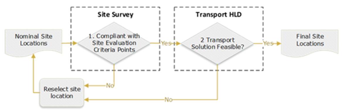
Figure16 Site location validation methodology
- The first step is to validate site evaluation criteria points (addressed in section 2.5 and summarized in Site Location Validation Questionnaire). If any of those dont comply, a new site location must be selected for the studied site.
- If site evaluation is successful, the transport team needs to validate the site location in terms of the transport solution feasibility. If site location is not feasible (due to any reason given by the transport team) a new location must be selected.
If the studied site location is compliantwith both site survey and transport evaluation, then it will be considered asthe final location for that site. This process must be followed for all plannedsites.
It must be noticed that if nominal sitelocations are based on previously defined locations, nominal locations areconsidered as the final ones.
Design Example
This step is not considered for the example asthe site survey wont be done.
Dependencies with other tasks
Prerequisites
4.2.9RF Equipment BOQGeneration
A RF equipment BOQlists all necessary RF equipment required to deploy a radio site. Its fed withthe overall equipment needed to deploy the network. Some items the RF equipmentBOQ must address are shown below:
A NaaS operator can use the RAN HLD Template thatcontains a BOQ format to create its own.
Design Example
The final step in the RAN HLD process is to generate a BOQ that summarizes the required radio equipment based on the selected configuration.
Following the final configuration displayed in Table 24, a BOQ for the design example is shown in Table 25. This initial BOQ doesnt consider backhaul equipment, power supplies, and installation miscellaneous that would be part of the low-level design.
Table 25 Design example bill of quantities
Dependencies with other tasks
Prerequisites
4.3NaaS Operator E2EProcess Definition
The NaaS operatorcan use the generic process design as a base to develop its own versionaccording to its limitations and constraints. A deep analysis of the processcan be performed to adapt the generic process.
Analyzing the provided generic processdesign, activities can be classified into two groups:
One-time activities Tasks tobe done only one time during the design process. These only require resourceconsumption at the beginning of the process. In the provided process, one-timeactivities are all activities except for RF configuration and site locationvalidation, which are part of the feedback activities.
Feedback Activities Tasks that can be made more than one time due tofeedback received from other modules. These will consume most resources duringthe design phase. In the provided process, feedbackactivities are RF configuration and site validation. External modules thatinteract with these processes are: site survey and transport HLD.
The approach presented in this section willfocus on continuous activities as they consume the majority of the resources. Someguidelines follow that the NaaS operator should consider to customize its ownprocess:
Preprocessing of one-time activities One-timeactivities should be done at the beginning of the process to refrain fromconsuming resources.
Its highly recommended that the NaaSoperator execute a critical path analysis over its process version to furtheroptimization. The methodology to perform a critical path analysis can be foundin the corresponding module.
5HLD Recommendation
Methodology to consolidate and generate afinal HLD recommendation.
5.1HLD RecommendationFormat & Structure
The main deliverable is the HLDrecommendation that contains the overall technical solution, basic designrules, technologies, and concepts required to describe RAN. The HLDrecommendation must contain the following aspects:
Overview A high-leveldescription that summarizes the RAN design.
RAN Solution Design Presentthe description of main scenarios to be implemented duringthe deployment phase.
RF Equipment BOQ Primary input for RF equipmentpurchase order generation.
5.2HLD RecommendationGeneration
Generation of the HLD recommendationfollowing the format and structure established. The NaaS operator can use the HLD Report Template asa reference to create its own version.
1. RAN Network LLD Introduction
Low-Level Design (LLD) for the Radio Access Network (RAN) refers to RAN equipment and antenna selection, detailed design of the base station configuration (setting azimuth and tilt values) and the parametrization of the Radio Access Technology (RAT). The RAN LLD impacts on the overall performance of the access network and is the last engineering step before deployment. This raises the necessity for the development of an LLD that efficiently integrates HLD inputs and NaaS Operator requirements into a cost-effective design.
The RAN LLD Module provides the NaaS Operator with instructions for RAN equipment evaluation and selection as well as background information and methodologies to elaborate a detailed design and parametrization of new base stations to be integrated into an existing network or in a region without existing sites. This module focuses on providing a generic end-to-end process flow that can be tailored to match the specific NaaS environment.
Main deliverables that the NaaS Operator will be able to generate through the use of this module are site Data Fills and Configuration Baseline, which are basic documents for the commissioning and integration of new radio sites. In addition, this module will guide NaaS Operator through the process of generating an LLD report to facilitate future network re-configuration and optimization.
1.1 Module Objectives
This module will enable a NaaS Operator to stand-up, run and manage a RAN LLD initiative. The specific objectives of this module are to:
- Provide an information base and fundamentals to perform the tasks associated with RAN LLDs.
- Provide detailed how-to instruction on the key RAN LLD engineering tasks.
- Provide an overview of the end-to-end RAN LLD process with instructions for tailoring to specific NaaS environments.
- Provide guidelines to develop a formal RAN LLD recommendation.
1.2 Module Framework
NaaS Runbooks Framework shown in Figure 1 displays the PlayBook Modules and their relationship to the RAN LLD.
The Strategic Plan & Scope and High-Level Network Architecture modules provide the business and technical context for the NaaS Operator and have direct impact and influence on many aspects of the Network Design.
The RAN LLD Module is included within the Network Design Area. It takes inputs from the RAN HLD and the output generated serves as the required input for the Civil & Power Design module.
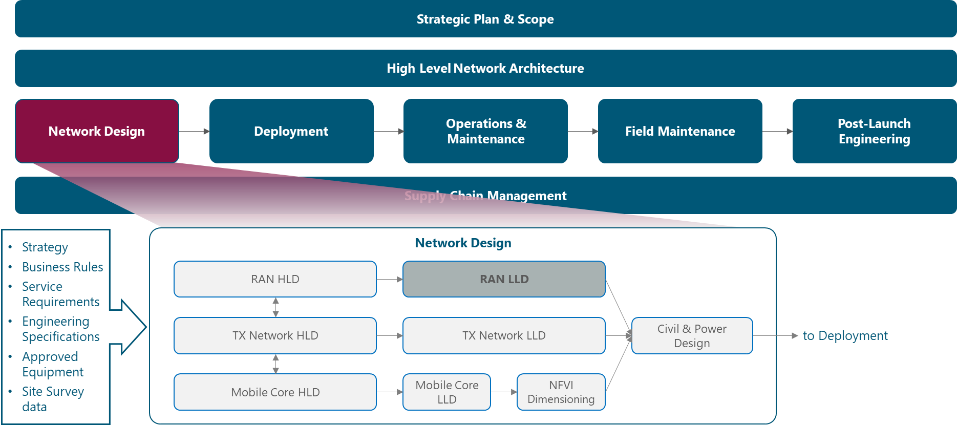
Figure 1. PlayBook Framework.
Figure 2 presents the RAN LLD functional view where the main functional components are exhibited. Critical module inputs are further described and examined in section 2.2. In addition, guidance and methodologies to execute the tasks included within each function are described in Section 3.
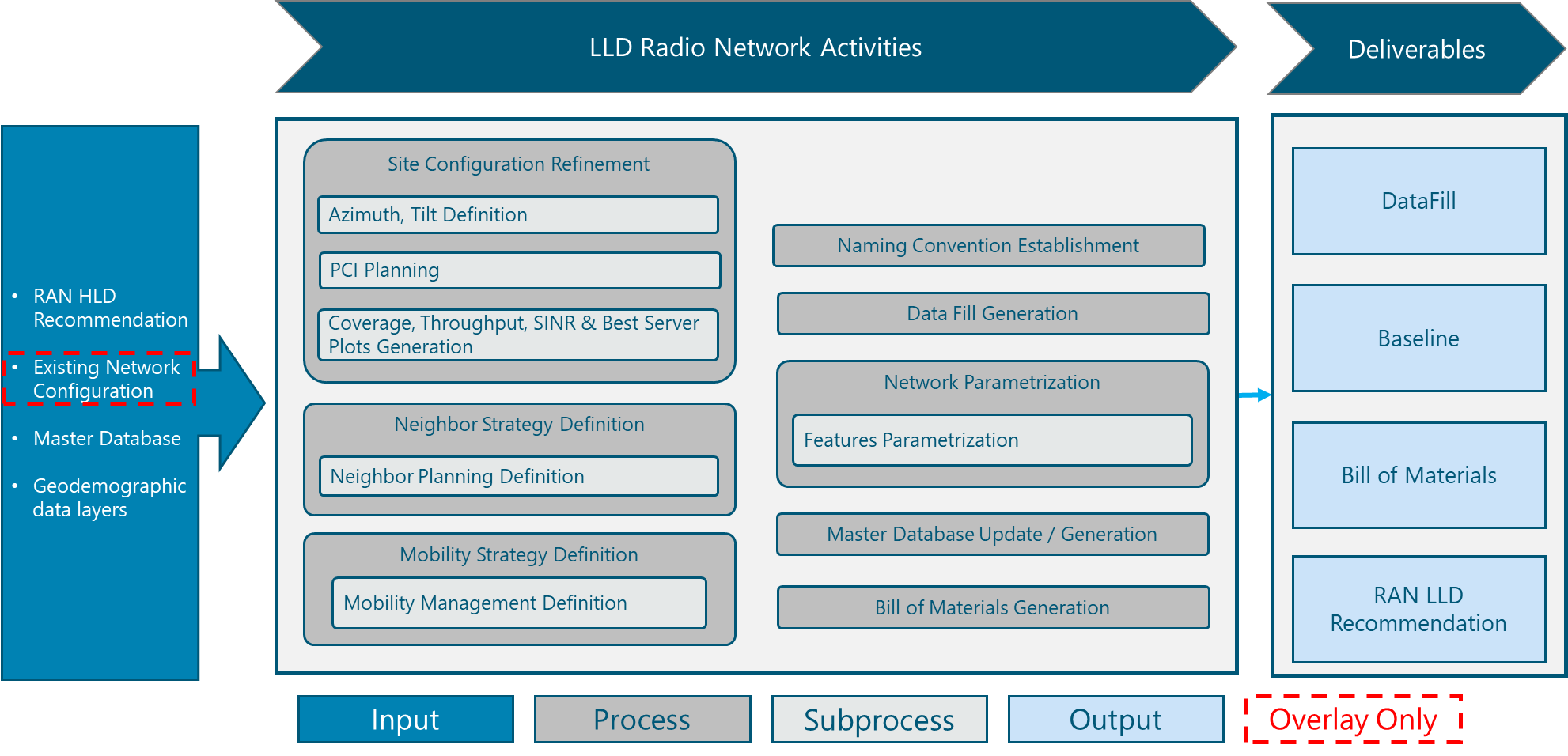
Figure 2. Overlay RAN LLD Module Functional view.
2 LLD Fundamentals
This section provides a general overview of the baseline concepts to develop an LLD RAN Design.
2.1 Low Level Radio Access Network Environment
Once the High-Level Design (HLD) process is carried out, the NaaS operator will have a general overview of the overall Deployment: number of sites and their configurations. The RAN Low-Level Design (LLD) process focuses on refining the RAN HLD proposed configurations and analyzing their performance by obtaining plots that will help the designer in finding opportunity areas to improve the performance of each site’s network. These analyses may involve certain iterations until the designer finds the configuration that maximizes performance results.
Additionally, during the LLD, the NaaS operator must select the equipment and establish the basic parameter to commission a RAN site. Such parameters will be introduced in section 2.3. These parameters will be consolidated in the Data Fill and Network Baseline, whose elaboration will be presented in sections 4.2.6 and 4.2.7 respectively.
RAN LLD is a crucial part of the design process as it sets the final configuration values of the RAN elements. A correct RAN LLD shall minimize optimization tasks and provide a quick time to market of the NaaS initiative, providing a good user experience from network launch.
2.2 Low-Level Radio Access Network Design Inputs Description
Table 1 presents a description of module input data and candidate sources required for a RAN LLD. Furthermore, the impact of each input on the design process is examined.
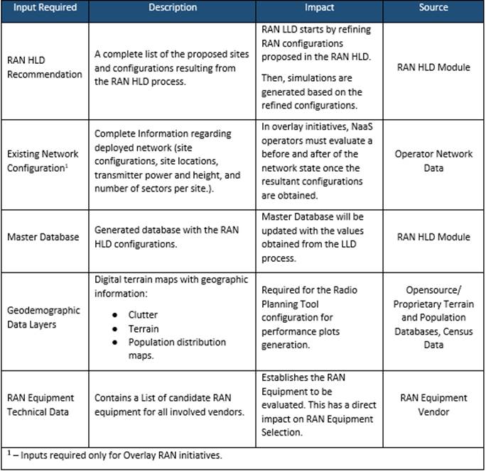
Table 1. Low-Level Design process inputs summary.
2.3 LTE Air Interface Fundamentals
Long Term Evolution (LTE) air interface is heavily influenced by the requirements for achieving high peak transmission rates, spectral efficiency, and being able to support multiple channel bandwidths (1.4, 3, 5, 10, 15, and-20 MHz) across several operational bands. For a complete table with 3GPP defined frequency bands, please refer to Annex A of the RAN Architecture Module. Figure 3 summarizes carrier bandwidths and spectrum bands used from a coverage and capacity point of view.
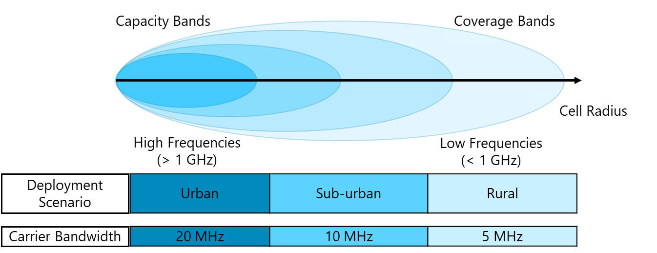
Figure 3.Characteristics of spectrum bands and carrier bandwidths.
The specific center frequency for each carrier is not pre-defined within each band. Thus, it is necessary to restrict the locations of the carrier centers for management purposes. With this objective, each carrier in an LTE network is identified within its own frequency band by an attribute called E-UTRAN Absolute Radio Frequency Number (EARFCN).
EARFCN is used to determine the exact frequencies for downlink (DL) and uplink (UL) transmission.
Estimation of the Downlink and Uplink frequencies (![]() and
and ![]() , respectively) is made through the following equations:
, respectively) is made through the following equations:
|
|
(Eq. 1) |
|
|
(Eq. 2) |
Where:
 Downlink EARFCN
 Uplink EARFCN
 Low part of the downlink band
 Low part of the uplink band
 Offset used to calculate downlink EARFCN
 Offset used to calculate uplink EARFCN
Table 15 in Annex A displays values required for ![]() and
and ![]() computation.
computation.
Equations 1 and 2 can be used to obtain the EARFCN from NaaS Operator DL and UL frequencies. The following steps can be used to determine the EARFCN of a given operating band and operating cell bandwidth (both defined in the RAN Architecture Module).
- Considering cell bandwidth, locate the center of the spectrum block available. Two cases can rise from this step:
- Cell bandwidth is exactly the bandwidth available in the available block.In this case, the cells center frequency must be located exactly at the middle of the available bandwidth as shown in Figure 4.
- Cell bandwidth is smaller than the available bandwidth.
In this case, the cell center must be placed in such a way that the end of the cell bandwidth meets the end of the operating band bandwidth as shown in Figure 5. - Once cell centers are known, the EARFCN calculator widget can be used to compute the corresponding EARFCN for both DL and UL frequencies.
Figure 4. Frequency center location when cell bandwidth and spectrum block bandwidth are equal.
Figure 5. Frequency center location when cell bandwidth and operating band are different.
The LTE air interface implements several techniques to fulfill the high transmission rates and high spectral efficiency requirements, among which, the most important are:
These techniques have a major impact in how radio resources are distributed among the air interface. Deeper insight into the specifics of the LTE air interface can be found on the LTE Air Interface basics primer.
Finally, there is an important aspect of the air interface that is used to achieve user equipment (UE) synchronization to the eNodeB or base station: synchronization signals which are the Primary Synchronization Signal (PSS) and the Secondary Synchronization Signal (SSS).
A User Equipment (UE) wishing to access the LTE system follows a cell search procedure that includes a series of synchronization stages by which the UE determines the time and frequency parameters that are necessary to demodulate downlink signals, to transmit with correct timing and to acquire some critical system parameters. The detection of the PSS and the SSS allows the UE to complete time and frequency synchronization and to acquire basic system information such as Cell Identity, decode broadcast channel, etc.).
The combination of the different values of PSS and SSS produce a parameter named Physical Cell Identity (PCI) which is a cell identifier. There are 504 unique PCIs available. These identities are organized in 168 groups of 3. A PCI is thus uniquely defined by the number ![]() in the range of 0 to 167 (PCI group) and the number
in the range of 0 to 167 (PCI group) and the number ![]() in the range of 0 to 2. Then, a PCI is built following the next equation:
in the range of 0 to 2. Then, a PCI is built following the next equation:
|
|
(Eq. 3) |
PCI parameter is a key part during LTE planning as it uniquely identifies between cells in the network and collision between cells with the same PCI will be reflected in service degradation. Instructions for its planned allocation will be given in section 3.1.2.
There exist other Low-Level parameters that are part of the configuration of the RAN equipment. However, these parameters are out of the scope of this section as the general recommendation for NaaS operators in the early stages is to follow the default recommendation provided by the RAN equipment vendor.
2.4 Antenna Basics
Antennas are one of the main building blocks of a base station as they transform electrical signals into electromagnetic waves and vice versa allowing for wireless communication. Antennas are considered to have a reciprocity property, which means that an antenna will maintain the same characteristics regardless if it is transmitting or receiving. Main antenna characteristics to be considered during a mobile network deployment are:
- Antenna Directivity and Gain
- Omnidirectional antennas: These antennas radiate in all directions (360 coverage) in the horizontal plane. Omni directional antennas are most used in small cell deployments for indoor or low coverage/capacity scenarios. Representation of an omni directional antenna is shown in Figure 6.
- Directional antennas: These antennas concentrate their energy on a single direction, making them ideal when coverage is required on a specific area of the whole region. Representation of an omni directional antenna is shown in Figure 7.
- Radiation Pattern and Antenna Beamwidth
- Antenna Tilt
Directivity is the ability of an antenna to focus energy on a particular direction when transmitting, or to receive energy better from a particular direction when receiving. This means that it is possible to use a directive antenna to concentrate the radiated signal in the wanted direction. Antennas can be classified into two types regarding their directivity:
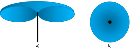
Figure 6. Omnidirectional Antenna. a) Side View, b) Top View.
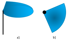
Figure 7. Directional Antenna. a) Side View, b) Top View.
The gain of an antenna is a rather complex concept that can be summarized as the amount of energy radiated in an specific direction compared to the energy that an ideal isotropic antenna would radiate in the same direction when driven with the same input power. Antenna gain results in an increase in the radiated power due to energy focusing.
Therefore, a relationship between antenna directivity and gain can be observed: the more directive the antenna is, the higher its gain, thus, the greater distance it will be able to achieve in a particular direction. On the other hand, an antenna with low directivity (omnidirectional) will have a lower gain.
Radiation pattern describes how the strength of the radiated energy is distributed across all antenna directions. The radiation pattern is also a reception pattern, due to the reciprocity principle of antennas.
As can be assumed, the radiation pattern is a three-dimensional representation of the radiated energy, however, the two must useful views are the vertical view (like if seen the antenna from one side) and horizontal view (like if seen from top of the antenna). Figure 8 shows radiation partners for an omnidirectional antenna while Figure 9 shows radiation pattern for a directional antenna.
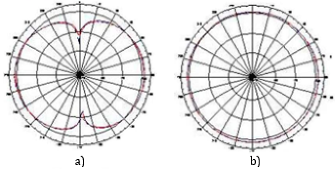
Figure 8. Omni Directional Antenna radiation pattern. a) Horizontal pattern, b) Vertical pattern.
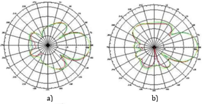
Figure 9. Directional Antenna radiation pattern. a) Horizontal pattern, b) Vertical pattern.
Size of the horizontal and vertical views are measured in degrees and are called Horizontal and vertical beamwidth. Commonly, horizontal beamwidth can span from 45 to 85, depending on the deployment scenario: 75 to 85 antennas for two sector sites and 65 antennas for three sector sites.
Regarding vertical beamwidth, 15 is a common value used for most mobile networks.
Antenna tilt represents the inclination of its vertical radiation pattern with respect to its axis. There are two types of Tilt:
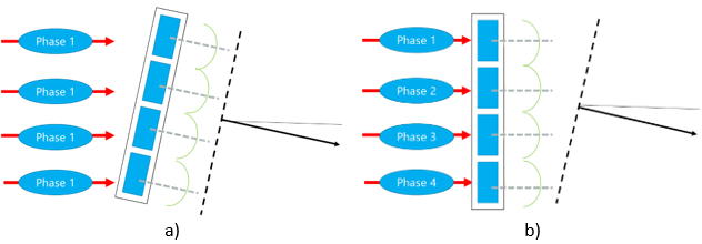
Figure 10. Antenna Tilting. a) Mechanical Tilt, b) Electrical Tilt
Final value for antenna tilt is the addition of both mechanical an electrical tilt.
3 Functions & Methodologies
This section presents various methodologies to perform critical tasks/subtasks involved in the RAN LLD process. Once NaaS operators have gone through these methodologies, they will be able to perform all activities in the End-to-end process flow.
3.1 Configuration Refinement
In order to have a radio configuration completely defined, it is required to define sector azimuth, tilt, and Physical Cell Identity (PCI) for each cell. This section will provide a methodology to define these parameters.
3.1.1 Azimuth and Tilt Definition
Setting antenna parameters such as azimuth and tilt is a key step in the network design as they will impact on the RF coverage and signal quality at a user equipment (UE). The azimuth of an antenna refers to the orientation (in degrees) of the antenna where the radiation lobe is pointing to. On the other hand, antenna tilt refers to the inclination of the antenna in order to get the desired coverage radius. These parameters are shown in Figure 11.
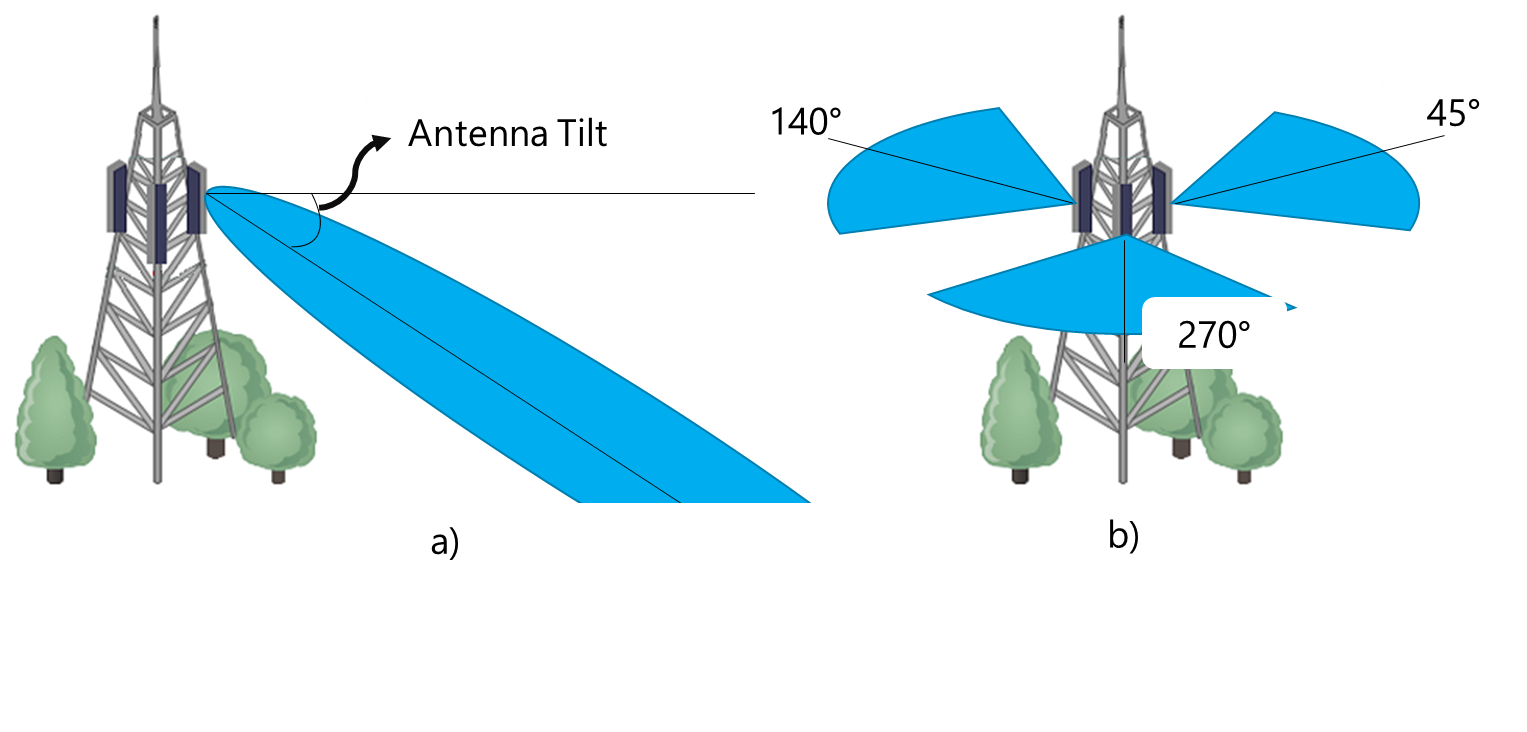
Figure 11. RF Configuration. a) Antenna Tilt, b) Antenna Azimuth.
As a result of the RAN HLD process, a high-level network dimensioning is obtained. This dimensioning provides the number of required sites and their configuration to cover an area: location, transmitter height, transmitter power and number of sectors per site. This HLD RAN configuration can be modified during the Site Configuration Refinement step (discussed in section 4.2.2) to achieve or improve network performance based on final selection of RAN equipment which is addressed in in Section 4.2.1.
However, to analyze RAN configuration performance, additional parameters are required. These parameters are antenna azimuth and tilt.
The process to establish these parameters is shown in the following steps.
- Antenna Azimuth: If the site has an omnidirectional antenna, it is not necessary to assign an azimuth as the antenna provides 360 coverage by definition. For sector antennas, the azimuth must be established in such a way as to cover the areas and coverage objectives established in the HLD: schools, hospitals, government buildings, etc.
- Antenna Tilt: Based on the coverage radius calculated in the HLD, it is possible to determine the antenna inclination required to achieve the target coverage. Typical tilt values range from 0 to 5 and its definition can be done following two recommendations:
- An antenna can be given a 0 tilt if the site or the sector is isolated, this means, it has no other site or sector near to it. In this way, coverage can be maximized. In particular, 0 tilts are commonly used in rural environments to expand coverage as much as possible.
- When the site or sector is not isolated or is placed on a very high location, tilt must be > 0 so it doesnt interfere with neighbors coverage. However, tilts should be kept below 5 to preserve some coverage overlap for handover.
To set the azimuth of a site, the site needs to be located in the GIS tool (e.g. Google Earth). Then, identify the coverage area or the specific coverage objective as shown in Figure 12.
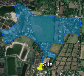
Figure 12. Coverage area example.
Designer must take care not to overlap antenna azimuths of antennas in the same site. Separation between antenna azimuths must be of at least equal to the horizontal beamwidth.
Finally, using the distance tool, measure the direction from the site to the center of the coverage area and take note of the required degrees as shown in Figure 13. This value will be the azimuth required for the antenna.

Figure 13. Establishment of the antenna azimuth using Google Earth.
Using the HLD results, selected equipment characteristics and the GIS tool, antenna mechanical tilt can be computed as displayed in Figure 14.
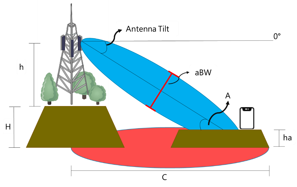
Figure 14. Required information for antenna tilt calculation.
Where:
First step is to compute total antenna height (TH) as follows:
|
|
(Eq. 4) |
Next, difference between Total Height and area height is computed:
|
|
(Eq. 5) |
Angle of incidence can be obtained from:
|
|
(Eq. 6) |
In order to obtain the result in degrees, the angle of incidence must be converted from radian as shown:
|
|
(Eq. 7) |
Finally, antenna tilt is obtained using the following equation:
|
|
(Eq. 8) |
Where:
![]() Is the antenna electrical tilt.
Is the antenna electrical tilt.
NaaS Operator can use the Antenna Tilt Calculator widget for this task. If computed tilt is > 5, it is recommended to low it down to 5.
Overlapping areas between adjacent sites is required for mobility purposes (handovers). However, overlapping must not be grater that 20% of the cell coverage area in order to avoid too much interference and the ping-pong effect in the UE.
3.1.2 Physical Cell Identity Planning
LTE considers 504 unique physical cell identities (PCIs) organized in 168 groups, each one containing up to 3 PCIs.
Cells with the same PCI must be isolated as much as possible (distance between two cells with the same PCI must be maximized) in order to ensure that the UE never simultaneously receives the same identity from more than a single cell.
There are several ways and algorithms to distribute the PCIs in a network, however, in rural environments that require few sites to provide coverage and / or the distances between sites are very large, the allocation of PCI can be simplified to comply with the following recommendations:
Figure 15 displays an example of PCI allocation.
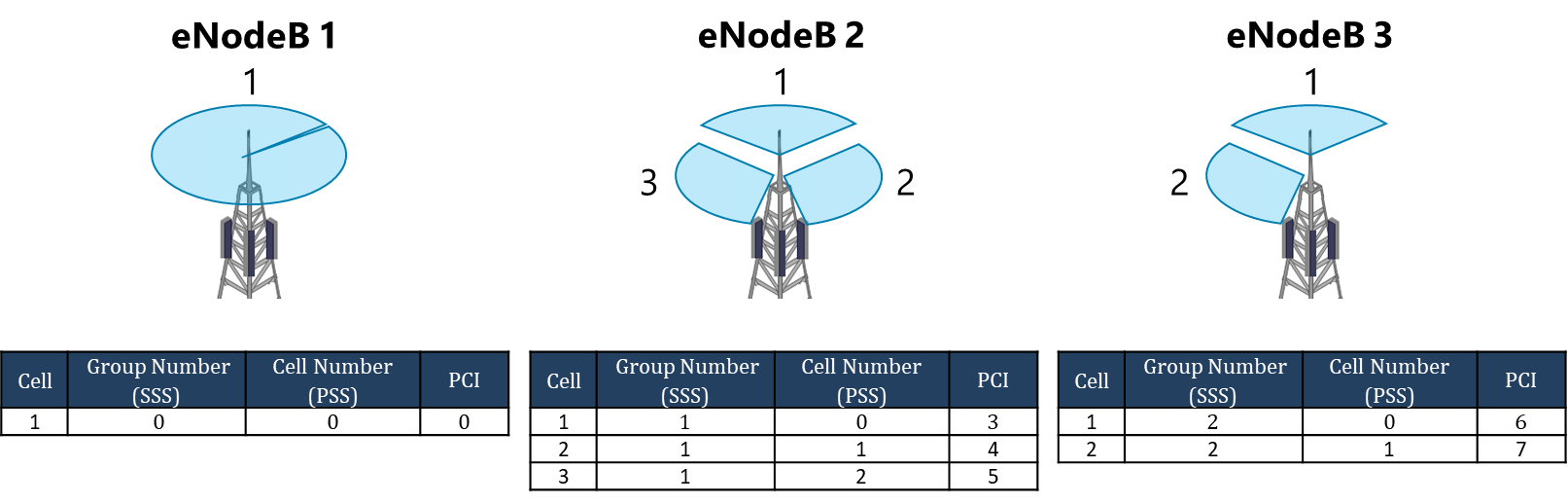
Figure 15. PCI Allocation example.
3.2 Radio Planning Tool Configuration
A Radio Planning Tool (RPT) helps the NaaS operators to generate the required performance plots (coverage, throughput, and signal quality) required to analyze the performance of the network and see which areas can be enhanced. Plots will also allow to define neighbor cells by showing which sites present overlapping coverage. If at this point, the NaaS Operator has not selected an RPT, please refer to Section 3.6 of the RAN HLD module.
Budget constraint NaaS Operators may not have access to an RPT. In such cases, the NaaS Operator can work only with HLD link budget results and refined configurations which will be enough to deploy the site but with the risk of sub-optimal performance.
Each RPT will have its own steps for project configuration. However, a generic process for RPT configuration is described below:
3.3 Coverage, Throughput, SINR and Best Server Plots Generation
Radio Planning Tools can generate several performance plots (depending on the RPT). However, there are some plots that are recommended to be generated in order to have an overall view of the network performance:
- Coverage plots: These plots show the signal strength across the target coverage area. LTE Reference Signal Received Power (RSRP) is the indicator to be plotted to analyze coverage.
- Throughput Plot: RPT can simulate the throughput that can be achieved throughout the coverage area, enabling the identification of areas that will struggle in terms of user experience. Figure 17 displays an example of a Throughput plot.
- Signal Quality Plot: Sometimes an area may appear to be correctly covered by the base station, however, the users may experience bad signal quality, which reflects on connection drops due to interference from other cells. For this reason, it is important to analyze the Signal to Interference plus Noise Ratio (SINR).
- Best Server (Overlapping) Plot: Sometimes, the area which is intended to be covered by one cell may be covered by another cell too (interfered). In such cases, SINR is low in the desired region. Best Server plot shows the region for which each cell provides the highest SINR. This plot is useful to study overlapping between cells of the same site or from other sites. Figure 19 displays an example of a Best Server plot.
- Electrical Tilt
- Mechanical Tilt
- Transmitter Power
- Antenna Height
- Site Location
- Every RPT shall have a menu to select a plot type. The required plot to be generated in this step must be selected.
- Generate a Baseline plot of the existing network (in an overlay scenario). This will show a before and after state of the network.
- Set the color patterns and thresholds required for each plot.
- Use the options provided by the RPT tool to generate the configured plot.
- Once the simulation is finished, the result can be exported in a format such as image (jpg), table (xml) or GIS document (kml).
As a reference, Table 2 displays a relation between RSRP ranges and signal strength.
|
RSRP |
Signal Strength |
|
>-80 dBm |
Excellent |
|
-80 dBm to -90 dBm |
Good |
|
-90 dBm to -100 dBm |
Fair |
|
-100 dBm to -110 dBm |
Poor |
|
<-115 dBm |
No Signal |
Table 2. LTE RSRP reference values.
Figure 16 displays an example of a coverage (RSRP) plot.
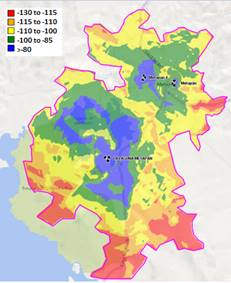
Figure 16. LTE Coverage (RSRP) plot example (values in dBm).
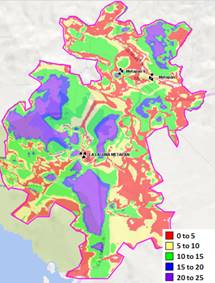
Figure 17. LTE Throughput Plot (values in Mbps).
As a reference, Table 3 displays a relation between RSRQ ranges and signal quality.
|
RSRQ |
Signal Quality |
|
>-10 dBm |
Excellent |
|
-10 dBm to -15 dBm |
Good |
|
-15 dBm to -20 dBm |
Fair to Poor |
|
<-20 dBm |
No Signal |
Table 3. LTE RSRQ reference values.
Figure 18 displays an example of an SINR plot.
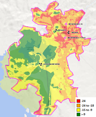
Figure 18. LTE Signal Quality (SINR) example (values in dB).
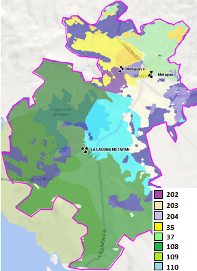
Figure 19. LTE Best Server Plot (values are PCIs).
Performance plots are useful as they serve to find areas where the configuration can be improved. For instance: a region covered by a single site can present acceptable coverage values, but it can suffer low SINR due to interference with adjacent sites. This will be displayed as an unwanted overlapping between two sites that can degrade user experience. In such cases, site configuration must be modified to reduce the overlapping. The following steps are recommended to be followed until performance plots provide an acceptable result:
Deeper plot analysis will be done as part of the design example shown in section 4.2.1.
Each RPT will have its own steps for plot generation. However, a generic process for the generation of the performance plots is shown below:
3.4 Neighbor Planning Definition
Neighbor planning involves the identification of the adjacent cells for a specific radio element. These adjacencies are used to inform the UE the cells to search for when completing handovers and cell reselections. In general, UEs are limited to the mobility routes defined by the neighbor list and missing neighbors can cause connections to drop.
This section provides instructions for manual neighbor management. However, some equipment models provide Self Organizing Network (SON) functions for an automatic neighbor management like the Automatic Neighbor Relationship (ANR) functionality. The importance of SON functionalities increases when the deployment involves a high number of sites which are close to each other. However, in rural environments, where sites tend to be far from each other or completely isolated, the manual procedure is enough for the neighbor planning task.
Each cell neighbors must be defined by following the next steps:
- Assign a number (1,2 or 3) clockwise to each sector (in case it is an omnidirectional site, only number 1 will be assigned) as summarized in Figure 20.
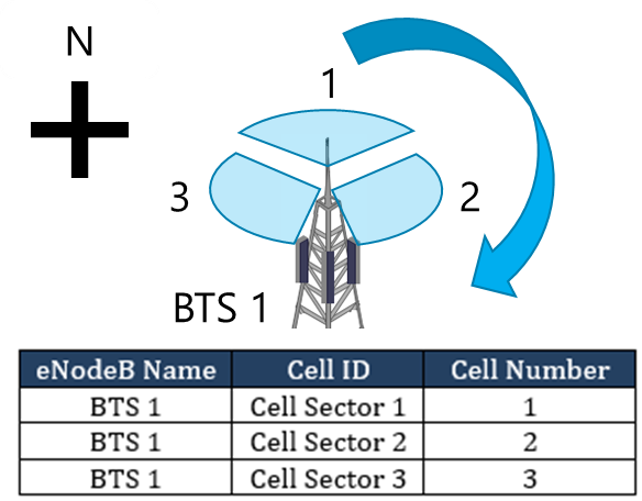
Figure 20. Cell numbering.
- Co-site: Assign co-site neighborhood (on the same site) within the same site following an ascending order. Figure 21 displays an example of Co-site neighbor definition.
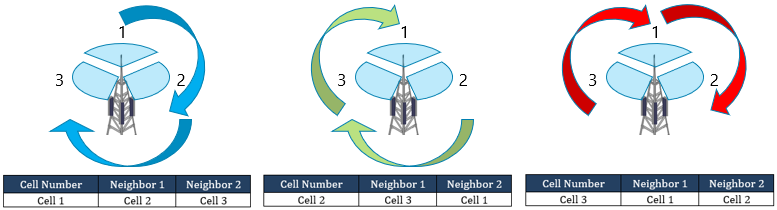
Figure 21. Co-site neighborhood definition.
- Inter-RAT Scenario: In the case that other RATs exist at the same site, NaaS operators must review how priority is being made on the existing RATs. Then, new cells must be configured for Inter-RAT relations. Figure 22 shows an example of inter-RAT relations definitions in a 3G +LTE RATs in the same site.
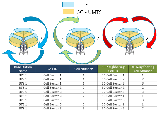
Figure 22. Inter-RAT co-site neighborhood definition.
3.5 Mobility Management Definition
Mobility is an important procedure to ensure that users can move freely within a network while keeping connectivity. The LTE mobility can be divided in:
Figure 23 summarizes LTE mobility scenarios.
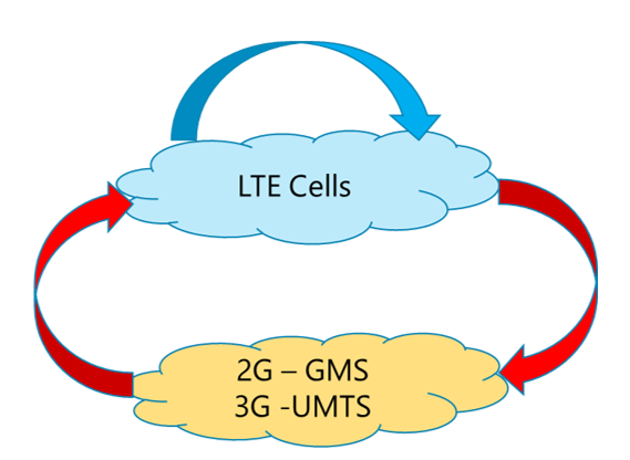
Figure 23. LTE Mobility scenarios summary.
The main task of mobility management is to establish priority values for each cell. Priority ranking method is used in mobility management to assign each carrier a number (ranking) which helps the UE to select an adequate cell to attach to. Ranking logic may vary from vendor to vendor; however, they usually follow the same logic: lower ranking means lower priority and higher number means higher priority. Most cases, ranking goes from 0 to 9.
The following subsections will provide guidelines to define priority rankings for mobility management for both Intra-LTE and Inter-RAT strategies based on NaaS Deployment scenarios.
3.5.1 Intra-LTE Mobility Rules Definition
Intra-LTE mobility can be classified in two:
Most rural environments are deployed with one cell per sector, in consequence, all cells must have the same priority in order to guarantee a smooth mobility between cells (in the same site or in different sites). As a best practice, it is recommended to set a priority lower than the maximum allowed (i.e. 7) in order to leave space for capacity expansions.
3.5.2 Inter-RAT Mobility Rules Definition
In the cases where CSFB is enabled, it is necessary that the UE returns to LTE once the voice connection with 2G or 3G has ended. In order to achieve this behavior, a low priority must be set in the 2G / 3G cells and a high priority for LTE cells. In such cases, priority ranking is used to ensure that devices reconnect to LTE (highest priority) from 2G or 3G (lowest priority) when LTE coverage becomes available.
Table 4 shows how to set priorities in an Inter-LTE scenario.
|
System Cell |
Value |
Comment |
|
LTE EUTRAN |
7 |
LTE shall be the highest priority RAT |
|
3G UMTS UTRAN |
6 |
UMTS shall be the middle priority |
|
2G GSM GERAN |
5 |
GSM shall be lowest priority |
Table 4. Priority ranking for Inter-LTE mobility.
3.6 Features Parametrization
Feature parametrization for NaaS deployments, should follow recommendations and guidelines provided by RAN equipment vendors as the details may vary from one vendor to another. However, in order to get a site on air, all the basic parameters can be set to the recommended value (as shown in each vendor documentation). This will assure that the network will be operating according to vendors best practices and recommendations, improving the time to get each site on air.
In addition, the steps below must be followed in order to assure that the network will be working as defined in the RAN Architecture module:
4 E2E Process Flow
This section presents a generic yet customizable end-to-end process flow to perform the Radio Access Low-Level design for the RAN.
4.1 End-to-end Process Overview
A generic end-to-end (E2E) process flow is shown in Figure 24. This process flow orchestrates general tasks and subtasks to perform the RAN LLD in a logical and well-structured sequence.
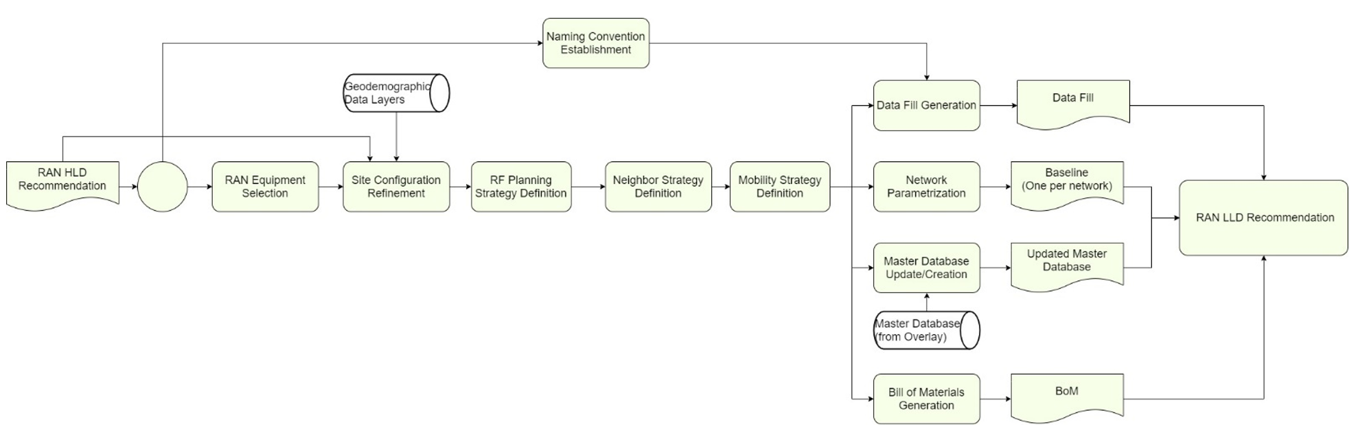
Figure 24. RAN LLD Generic E2E Process Flow.
RAN Low-Level Design starts with the RAN Equipment Selection is performed to evaluate between multiple vendor alternatives to define which options fits best in the NaaS Deployment, including eNodeBs (RRU and BBU) and antennas. Then, Site Configuration Refinement of the radio configurations proposed in the RAN HLD. Once configuration has been done, Performance plots are generated and analyzed to study network performance and, if required, modify radio configurations. After the analysis of the performance plots, the RF Planning Strategy for PCI allocation, Neighbor Strategy and a Mobility Strategy for each site and cell in the network can be defined. Naming Convention Establishment defines naming rules (nomenclature) to uniquely identify each eNodeB and each cell in the network.
Data Fill Generation will create a document containing eNodeBs basic information required for its integration. Network Parametrization focuses on the generation of a baseline that will be used to configure all sites in the network. Master Database Update will add the values resulting from the overall process to the existing Master Database built during the HLD process. Finally, HLD Bill of Quantity (BoQ) will be updated into a final Bill of Materials (BoM) containing the final equipment to be deployed at each site.
4.2 Step-by-Step Analysis
This section presents an examination of each of the steps involved in the E2E process to identify, isolate, and describe the range of implementation options on the path towards customization based on NaaS Operator requirements and constraints. Dependencies among tasks are addressed in the corresponding subsection.
4.2.1 RAN Equipment Selection
NaaS operators must perform the selection of the RAN Equipment from multiple vendor alternatives. The complete process to select the RAN Equipment is included within the Procurement Module (RFx Process Module). This section focuses on the technical aspects to perform the evaluation of transport equipment from different vendors.
From the technical perspective, Table 5 displays the typical requirements that the RAN equipment must satisfy which must be defined according to the final radio configuration.
|
|
Evaluated Characteristics |
|
Antenna |
Gain |
|
Electrical Tilt |
|
|
Horizontal beam width |
|
|
Vertical beam width |
|
|
Mounting Options |
|
|
Radio unit |
Transmitter power |
|
Operating Band |
|
|
Mounting Options |
|
|
Maximum number of supported sectors with a single Radio unit |
|
|
Operational Bandwidth |
|
|
MIMO Scheme |
|
|
Baseband |
Maximum Supported users (simultaneous RRC connections) |
|
Maximum supported throughput |
|
|
Maximum number of supported sectors |
|
|
Features support |
CSFB, VoLTE, C-RAN support |
|
Dimensions |
Equipment Dimensions and physical characteristics |
|
Power Requirements |
Power consumption profile |
|
Environmental Protection |
IP (Ingress Protection) certification |
|
Price |
Equipment price |
Table 5.Typical specifications to be evaluated in RAN equipment.
The decision to select the RAN Equipment is also affected by the financial constraints of the project. The final selection of the RAN Equipment is performed during the RFx process and in conjunction with the Procurement Team.
Additionally, the Naas operator can use the RAN Equipment Evaluation Matrix Template to support in the technical evaluation of different RAN equipment.
Design Example
Table 6 displays a comparison of two generic vendors as a matter of example (power consumption and prices are an assumption):
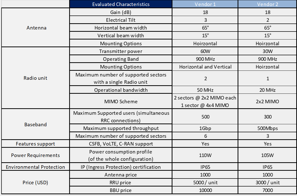
Table 6. Design Example RAN Equipment evaluation.
Based on the data above, vendor 1 has better performance in both Radio and Baseband units than vendor 2. However, these enhanced capabilities come with a higher price. In addition, as the NaaS Deployment is taking place on a rural environment, performance provided by vendor 1 is unnecessary and will not be exploited as it can be.
From this analysis it is concluded that configuration offered by vendor 2 suits better with the design example deployment.
4.2.2 Site Configuration Refinement
Refinement of the proposed configurations in the RAN HLD process is required to be done during the RAN Low-Level Design as it adds the required values for antenna azimuth and tilt of each site. The required data to compute these values, such as maximum transmitter power, antennas vertical beamwidth and electrical tilt is obtained from the specifications of the selected equipment in the previous step..
These values together with the ones obtained during the RAN HLD process (such as site coordinates, site height and transmitter power) are required to generate the performance plots. As mentioned in section 3.3, these plots will be used to analyze the site’s performance and make any required modifications if poor coverage, low quality or bad throughput are present.
Figure 25 displays the process to be followed for the generation of the performance plots and final site configurations.
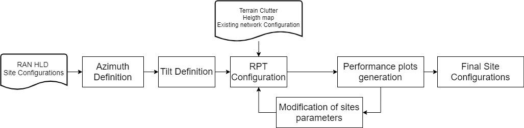
Figure 25. Performance Plots generation process.
With the proposed site configurations from the RAN HLD process, each site azimuths and tilts must be estimated following the methodology presented in section 3.1. Then, the RPT must be configured as sketched in section 3.2. Finally, performance plots must be generated to validate network performance.
However, as mentioned in section 3.2, NaaS Operatory may not have access to an RPT. If the deployment area is in a rural environment or no overlapping zones coverage are defined (sites close to each other), then NaaS Operator may work only with the defined azimuths and tilts using the GIS tool.
After plot analysis, the designer may decide to change site parameters (azimuth, tilts, height, etc.) if the current configuration is failing to deliver appropriate results. Bad performance results can be:
In such cases, new configurations must be proposed generating new performance plots until acceptable results are obtained. This process may represent a huge time investment but is of vital importance as these results will represent the final site configurations and the results must be good as possible in order to maximize network performance.
In order to show the implementation of the network design process, a Design Example is developed throughout all the steps of the process.
Design Example
Input for this example is composed by the three target coverage areas shown in Figure 26.
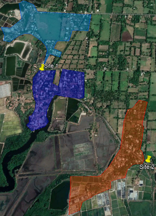
Figure 26. Design Example Coverage Areas and Proposed Sites Location.
As part of the inputs, the RAN HLD defines two sites to cover the desired areas. Table 7 displays HLD configurations of each site.
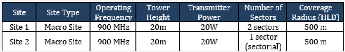
Table 7. Design Example Site Configurations.
Azimuth Definition:
Using Google Earth, azimuth for each site is obtained as depicted in section 3.1.1. Figure 27, Figure 28, and Figure 29 display the results for the Design Example.
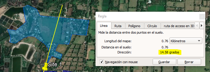
Figure 27. Sector 1 / Site 1 Azimuth definition for first coverage area.
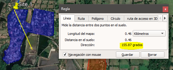
Figure 28. Sector 2 / Site 1 Azimuth definition for second coverage area.
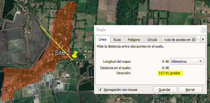
Figure 29. Sector 1 / Site 2 Azimuth definition for the third coverage area.
Azimuth values for each site are shown in Table 8.
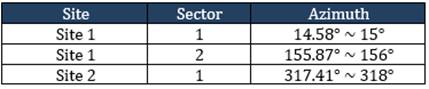
Table 8. Design Example Azimuth values.
Tilt Definition:
1) Site 1 has the following values:
2) Site 2 has the following values:
Complete site configuration is shown in Table 9.
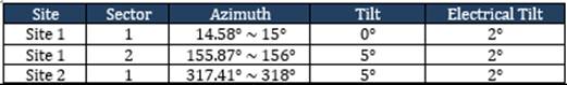
Table 9. Design Example complete site configurations.
For the design example, Atoll was used for the generation of the performance plots. Atoll was configured using a clutter and a heights map corresponding to the area under study (El Salvador) obtained from a specialized GIS company. Figure 30 displays the location of the design examples sites on Atolls configured project map.
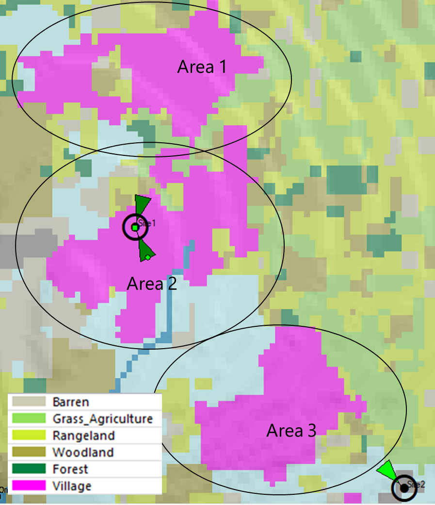
Figure 30. Design Example on the configured RPT.
Performance Plots Generation:
1) Coverage plots:
– Site 1, Sector 1:
Figure 31 displays the coverage plot for sector 1 of site 1. It can be noticed that with refined configuration, the region of interest is covered with good coverage values.
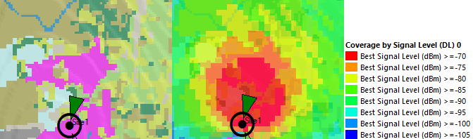
Figure 31. Coverage plot for Sector 1 of Site 1.
– Site 1, Sector 2
Figure 32 displays the coverage plot for sector 2 of site 1. As in sector 1, it can be noticed that sector 2 refined configuration good coverage values are obtained withing the required region.
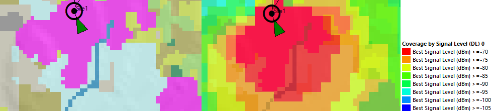
Figure 32. Coverage plot for Sector 2 of Site 1.
– Site 2, Sector 1
Figure 33 displays the coverage plot for sector 1 of site 2. This case also presents good coverage among the required coverage zone.
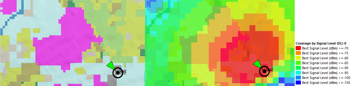
Figure 33. Coverage plot of Sector 1, Site 2.
Figure 34 displays a before and after of the three coverage areas.
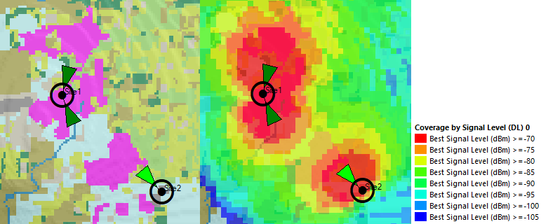
Figure 34. Design Example Coverage Plot comparison.
2) Throughput plot:
Figure 35 displays the throughput plot for the design example.
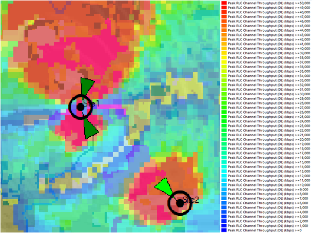
Figure 35. Design Example Throughput plot.
Overall throughput distribution on the desired areas appears to be well distributed among all the desired areas based on the throughput plot.
3) SINR and Best Server (Overlapping plots):
SINR plot for the design example is displayed in Figure 36.
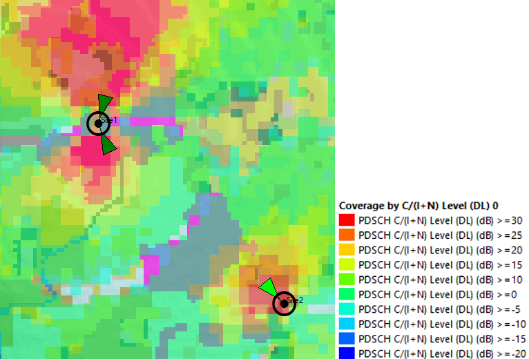
Figure 36. Design Example SINR Plot.
It can be noticed that SINR is high between sectors of site 1 (upper part of the image). However, poor SINR values are visualized inside Area 3, which lead to a bad overlapping as displayed in Figure 37.
As discussed in section 3.3, overlapping areas are required for mobility to be possible between sector. However, overlapping areas must be out of the main coverage area to avoid ping-pong effect in the UE.
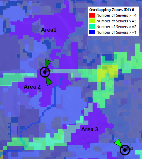
Figure 37. Design Example Best Server (Overlapping) plot.
It can be noticed that overlapping is happening across Area 3, which is an unacceptable result. A way of improving this situation is by modifying Sector1/Site2 electrical tilt by augmenting its tilt in order to mitigate impact from Sector2/Site1 into Area 3.
For this design example, electrical tilt was augmented from 2 to 4. Resultant coverage is shown in Figure 38.
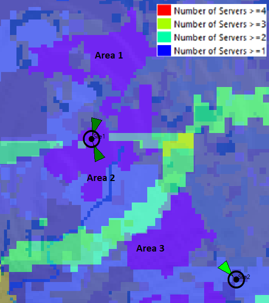
Figure 38. Modified Design Example Best Server (Overlapping) plot.
It can be noticed that, with the refined configuration, overlapping between Site1 and Site2 occurs almost out of both Area 2 and Area 3, which is an expected good result as each area will be covered by its corresponding site.
Final configuration for each site is shown in Table 10.
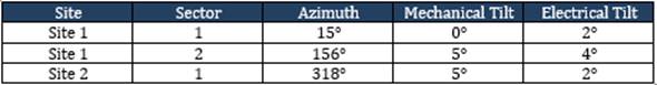
Table 10. Design Example final configuration results.
4.2.3 RF Planning Strategy Definition
PCI allocation may seem to be a random process due to the low number of sites/cells and the fact that in a NaaS Deployment sites tend to be isolated between them. However, it is highly recommended to always keep an order on the allocation of PCIs in order to have a management of used PCIs and available ones for any future expansion in the network.
Designer can follow the next steps for the allocation of the PCIs for each cell:
NaaS Operators can use the PCI Allocation Widget to generate and keep track of the used and available PCIs on its network.
Next step is to estimate cell EARFCN following the steps discussed in section 2.3.
Design Example
The example sites will be assumed to be the first in the network. Therefore, the first available groups will be chosen: group 0 and group 1.
The distribution of PCIs is shown in Figure 39.
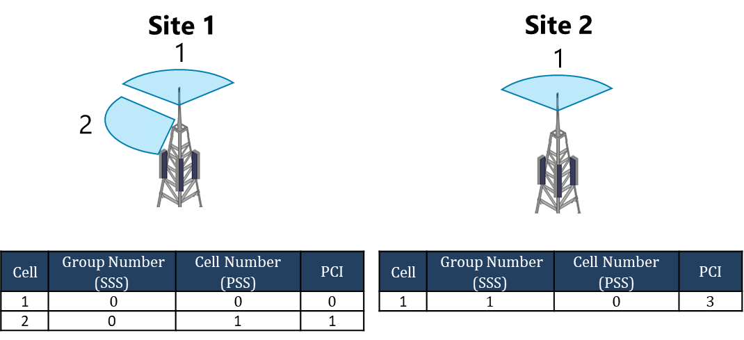
Figure 39. Design Example PCI Allocation.
EARFCN calculation:
– Band 8 (900 MHz)
– Cell Bandwidth: 10 MHz
Assuming that the whole band is empty, frequency centers will be located at the following locations:
Using the EARFCN calculator widget, the following EARFCN are obtained:
4.2.4 Neighbor Strategy Definition
The mobility strategy is defined based on the characteristics of the NaaS Deployment in terms of site adjacencies (how close are sites between them). From these characteristics, two cases can be defined:
Figure 40 shows an example of both cases.
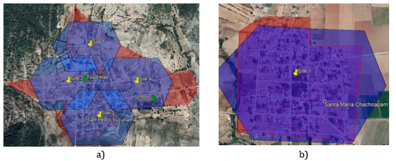
Figure 40. NaaS Deployment cases for Neighbor definition. a) More than 2 sites for a single region, b) One site for a single region.
Based on the defined cases, the methodology shown in Figure 41 may be followed to define the Neighbor strategy per site.
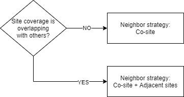
Figure 41. Neighbor Strategy methodology.
Design Example
Neighbor definition for the sites in the Design example is shown in Figure 42:
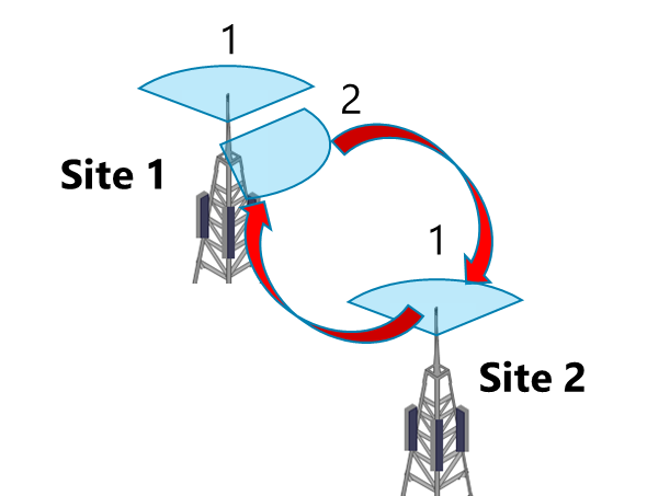
Figure 42. Design Example Neighborhood representation.
1) Site 1: As shown in Figure 43. Co-site neighborhood was defined between cells 1 and 2. In addition, cell 2 has an interaction between cell 1 of site 2, so this neighbor must be noted as well.
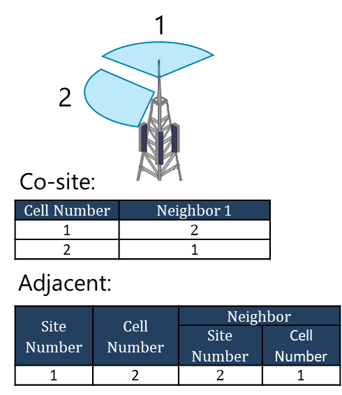
Figure 43. Design Example Neighborhood definition for Site1.
1) Site 2: As shown in Figure 44. Co-site is not present in this case; however, an adjacent neighborhood must be defined (now form site 2 perspective) between cell 1 of site 2 and cell 2 of site 1.
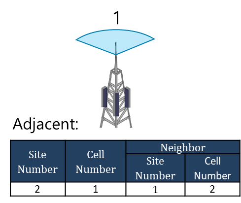
Figure 44. Design Example Neighborhood definition for Site 2.
4.2.5 Mobility Strategy Definition
The definition of mobility priorities will depend on the services to be offered and on network characteristics:
Design Example
Design example sites operate on a single frequency in the LTE System; thus, it is necessary to define only intra-LTE and intra-frequency interactions. Priority ranking for the design example will be set to 7 (below maximum value) as discussed in section 3.5.1.
4.2.6 Naming Convention Establishment
Every network requires that its main network elements (eNodeB and Cells) have unique names and identifiers for the maintenance, organization, and management of the network. The NaaS Operator needs to establish a Naming Convention (nomenclature) to define the following parameters (these parameters are generic, and the real name will depend on each vendor):
The creation of a nomenclature depends on the following two factors:
It is recommended that the nomenclature for the eNodeB Name and the Cell Name be similar and that they differ from each other by indicating in the Cell Name the sector number to which the cell corresponds. For example:
Design Example
For the design example, the following Naming Convention is defined for each of the parameters:
Where:
Table 11 displays nomenclature values to be used for naming.
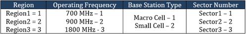
Table 11. Nomenclature values.
For the design example case, Naming for each element results as follows:
Site1:
Site2:
4.2.7 Data Fill Generation
Data Fill (DF) of a RAN site consolidates all the basic information of an eNodeB that will serve for its integration and turning up process. The basic information that a RAN DF must contain can be divided into the following sections:
A Data Fill can be built following two approaches:
NaaS Operator can use the Data Fill Template to generate its own version of a Data Fill.
Design Example
The final version of the Data Fill for the Design Example is included as part of the Data Fill Template.
4.2.8 Network Parametrization
Before turning on a site, multiple parameters must be configured (the amount of these depends on the seller). However, most of these parameters can be configured using the default values suggested by the vendor.
Parameters that must be considered with a special value depending on the network configuration are:
All the basic parameters and features to be activated are consolidated into a single Baseline Document. This Baseline is intended to serve as a base for the integration of all sites in the network.
NaaS Operator can build its own version of the baseline with the Baseline Template.
Design Example
The final version of the Network Parametrization for the Design Example is included as part of the Baseline Template.
4.2.9 Master Database Update
During the HLD process, a master database was generated, which contained the following parameters:
This master database must be updated with the results obtained through the LLD process:
NaaS Operators can use the same Master Database built during the HLD process and that was built using the Master Database Template.
Design Example
The final version of the Master Database for the Design Example is included as part of the Master Database Template.
Table 12, Table 13, and Table 14 display sections of the Master Database
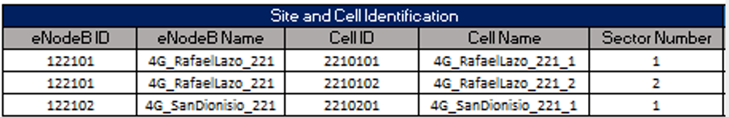
Table 12. Design example Site and Cell Identification section in Master Database.
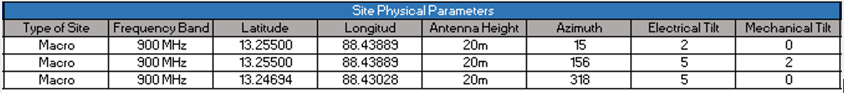
Table 13. Design example Site Physical Parameters section in Master Database.
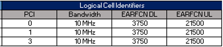
Table 14. Design example Cell Identifiers section in Master Database.
4.2.10 Bill of Materials Generation
As a result of the RAN HLD process, an initial Bill of Quantities (BoQ) must have been generated. Such BoQ should contain a high-level list of the required equipment based on the calculations made during the RAN HLD process:
In some occasions, the configuration proposed by the RAN HLD process can be modified once the RAN LLD process results are ready, i.e. a site initially considered with 2 sectors can be modified to only one sector after analysis of performance plots, etc.
In addition, once the RAN Equipment selection process is finished, a final BoM with the equipment to be used during the deployment phase can be built following the results from the RAN LLD process.
NaaS Operators can use the Bill of Materials Template as a base to create its own version.
Design Example
Figure 45 displays a snapshot of the bill of materials required for the design example configuration.
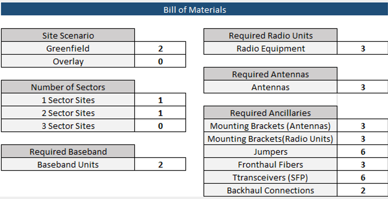
Figure 45. Bill of Materials snapshot for the Design Example.
For the design example, the following assumptions were made:
4.3 NaaS Operator End-to-End Process Definition
NaaS operators can use the generic process design as a base to develop its own version according to its limitations and constraints. In order to adapt the generic process a deep analysis of the process can be performed.
Analyzing the provided generic process design, activities can be classified into two groups:
The approach presented on this section will focus on continuous activities as they consume the majority of the resources. Following some guidelines that NaaS operator should consider in order to customize its own process:
Finally, it is highly recommended that NaaS operators execute a Critical Path Analysis over its process version for further optimization.
5 LLD Recommendation
This section presents a methodology to consolidate and generate a final LLD recommendation.
5.1 LLD Recommendation Format & Structure
The main deliverable from the RAN LLD process is the LLD recommendation which contains the overall technical solution, complete Radio Configuration, analysis conclusions and basic information for RAN implementation. The RAN LLD recommendation shall contain the following aspects:
5.2 LLD Recommendation Generation
Generation of the RAN LLD Recommendation following the format and structure established. NaaS Operators can use the RAN LLD Report Template as a reference to create its own version.
nbps;
RAN Civil and Power Design Introduction
Power and Civil Design for RAN Sites refers to the process performed to design a proper Power Solution and Sites Equipment Layout, considering as inputs the Site Characteristics, Network Equipment power requirements, RAN and Transmission LLD. An accurate Power and Civil design will achieve economically efficient Power Feed Solution and will facilitate forthcoming Installation and Maintenance Tasks.
The RAN Power Design assesses the Power Supply Options that suit the site scenario, which can be Grid or Solar. When the Power supply option has been established, the next step is to match the selected network components requirements with power systems capabilities, optimizing cost and protecting the NaaS Operator Hardware Investment. Once the Power Hardware is established, a Site Layout must be performed; the site layout indicates where the hardware must be installed, facilitating the forthcoming installation, maintenance, and future network upgrades.
The RAN Civil and Power Module provides the NaaS Operator with background information to aid in the selection and design of a customized Power System for their sites and guides NaaS Operators to prepare their Site Layouts that will define the position of all RAN & Power components in blueprints.
Main deliverables that the NaaS Operator will be able to generate through the use of this module are Power Equipment Bill of quantities and Blueprints for the Site Layout Equipment Component,
1.1 Module Objectives
This module will guide the NaaS Operator to accurately assess and dimension the Power Equipment for the RAN site and develop the Site Layouts that will define the equipment location, ensuring their right operation, and the installation of the equipment. The specific objectives of this module are to:
1.2 Module Framework
NaaS PlayBooks Framework shown in Figure 1 displays the PlayBook modules and their relationship to the Civil & Power Design for RAN sites Module.
The Strategic Plan & Scope and High-Level Network Architecture streams provide the business and technical context for the NaaS Operator and have a direct impact and influence on many aspects of the Deployment Stream.
The Civil & Power Design for RAN sites Module is included within the Network Design Stream. It takes inputs from the Mobile Core Architecture, the output generated serves as Guidelines for Core Equipment Installation.
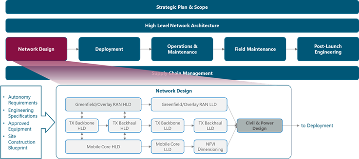
Figure 1. Network Design Framework.
Figure 2 presents the Civil & Power Design functional view where the main functional content of the module is exhibited.
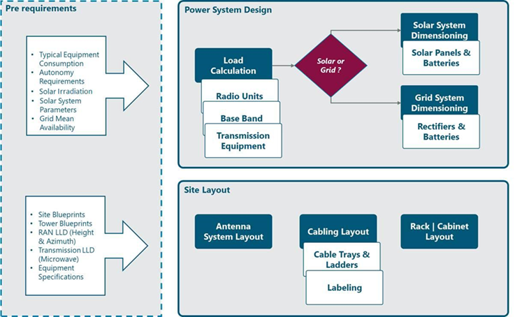
Figure 2 Civil & Power Design Functional View.
The rest of the module is divided into three sections. Section 2 is an introductory section, containing a high-level view of the power systems used for RAN sites, their main characteristics, and functions. Section 3 contains the key considerations used to design a power solution that properly fits the requirements for each site. Section 4 provides hands-on guidance for the Equipment Sites Layouts, including the Antenna System, Rack or Cabinet and Cabling.
2 Civil & Power Design Fundamentals
This section presents a description of the Civil & Power Design process including an analysis of the benefits to perform the Power System Design and Site Layout, the main tasks and inputs of the process and the description of the two most common types of power systems in rural deployments: Solar & Grid.
2.1 Civil & Power Design Overview
The purpose of Civil & Power Design is to select and size the Power System depending on the RAN Site Power requirements, and to define the position of all the RAN equipment through a Site Layout. An optimal sizing of the power system and a properly performed Site Layout will protect the NaaS Operator investment as follows:
Figure 3 depicts the Civil & Power Design Process. The first step is to calculate the Power Consumption of the RAN site equipment, considering that each equipment has its own load characteristics. Then various types of power systems are assessed; for this module Grid and Solar systems are considered, as these are the most common for NaaS deployments.
The first option is to consider Grid power which is the commercial AC power network. The feasibility of this option will depend on the general availability and reliability of the Grid service and the compliance with engineering requirements. In case that the Grid service is not available or not reliable, Solar Power Systems will be considered, which is sized according to the power consumption and autonomy requirements. Solar Power System may result unfeasible under high load conditions; in this case, the RAN/TX design must be reviewed to reduce the power load of the site.
The outcome of a properly designed power system is a reliable and optimized solution that will feed the RAN sites with minimum service outage.
Once the power system and the RAN LLD has been established, the site layout can be defined. It will determine the equipments position at the site, following the RAN and Transport LLDs as well as engineering standards.
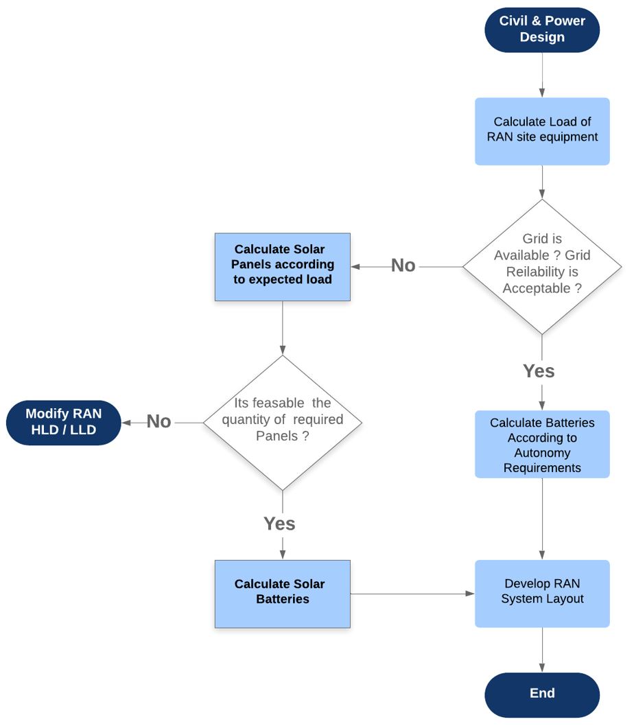
Figure 3. Civil & Power Process overview
2.2 Civil & Power Design Inputs Description
There is a wide variety of options to perform a Civil and Power Design, so to narrow them, some inputs have to be defined at the beginning of the design process. Table 1 below list the inputs of Civil & Power Design, show the impact on the overall process and its possible sources.
|
Input Required |
Description |
Impact |
Source |
|
Equipment Power consumption (W), Average Load or Maximum Load |
Power Consumption of RAN Site Equipment including RRU, Baseband, and transport equipment. |
Required to determine the total load to be supported by Power System Elements |
Network Equipment Vendor Specifications |
|
Grid Power Equipment Specifications |
Specifications of all Power Equipment: AC INPUT: ● Voltage Range ● Frequency ● Maximum Current DC OUTPUT: ● Voltage Range ● Maximum Power ● Maximum Current ● Peak Efficiency |
Required to properly size and select the Power System Elements |
Vendor Specifications |
|
Battery Specifications |
Specifications of the batteries for the Power System: ● Capacity (Ah) ● Self discharge time in % ● Battery Operative Voltage |
Required to properly size and select the batteries in the Grid or Solar Power System |
Vendor Specifications |
|
Solar Power Equipment Specifications |
● Solar Panel Nominal Power ● Output Voltage The Peak Power of a Solar Panel, regardless of the location |
Required to properly size and select the Solar Panels in the Solar Power System Elements |
Vendor Specifications |
|
Solar Irradiation |
Solar Irradiation received in Sites location. |
Used to dimension the number of solar panels. |
https://globalsolaratlas.info/map |
|
RF Equipment Dimensions & Weight |
Dimensions and weight of the RF equipment: ● Base Band ● RF Unit ● Antenna |
Required to define the Site Layout |
Vendor Specifications |
|
Site Survey Reports |
Inspections of physical sites to gather relevant information (e.g. equipment inventory, photographic documentation). |
Required to define the Site Layout for existing sites |
Vendor Specifications |
|
Site Engineering |
Contains detailed blueprints corresponding to each specific Site deployment of tower and bird eye view of the site. |
Required to define the Site Layout for greenfield sites. |
Site Construction Contactor |
Table 1 Input description of Civil and Power Design for RAN sites
2.3 Grid Power System Overview
A Grid power system is the set of equipment that takes electric energy from the public alternating current (AC) network and transforms it to direct current (DC) which is required to power the equipment at RAN sites. Modern grid networks are a reliable source of power, offer less outage duration and few power quality disturbance therefore when it is available the grid network is the preferred option to feed a RAN site as it ensures network service continuity at an acceptable cost.
A Grid Power System for a RAN site consists of four basic elements, shown in the schematic of Figure 4:
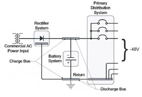
Figure 4 Simplified Schematic of the Grid Power System for RAN sites
Components in Figure 4 are described in the following paragraphs while further guidance for the sizing and selection of the various system components is provided in Section 3.
- Rectifiers. Elements in charge of converting the prime power source AC voltage to direct current (DC). Rectifiers serve three main purposes:
- Batteries. Energy storage devices that power the loads during AC power supply outages. Batteries are always connected to a busbar that connects the batteries from the load so there is no switchover time or interruption when the primary power source (and standby source, if equipped) fails or if the rectifier system fails.
- Power Distribution Units. Elements that provide central locations for feeding loads and for protecting circuit wiring. The distribution systems also provide a convenient way to isolate individual loads from each other during fault conditions. The primary distribution system has the first overcurrent protective device (either fuse or circuit breaker) between the discharge bus and the load. There are several solutions that Naas Operators may consider for their power system, commonly in low power rural scenarios, the PDU is installed within a Power Cabinet.
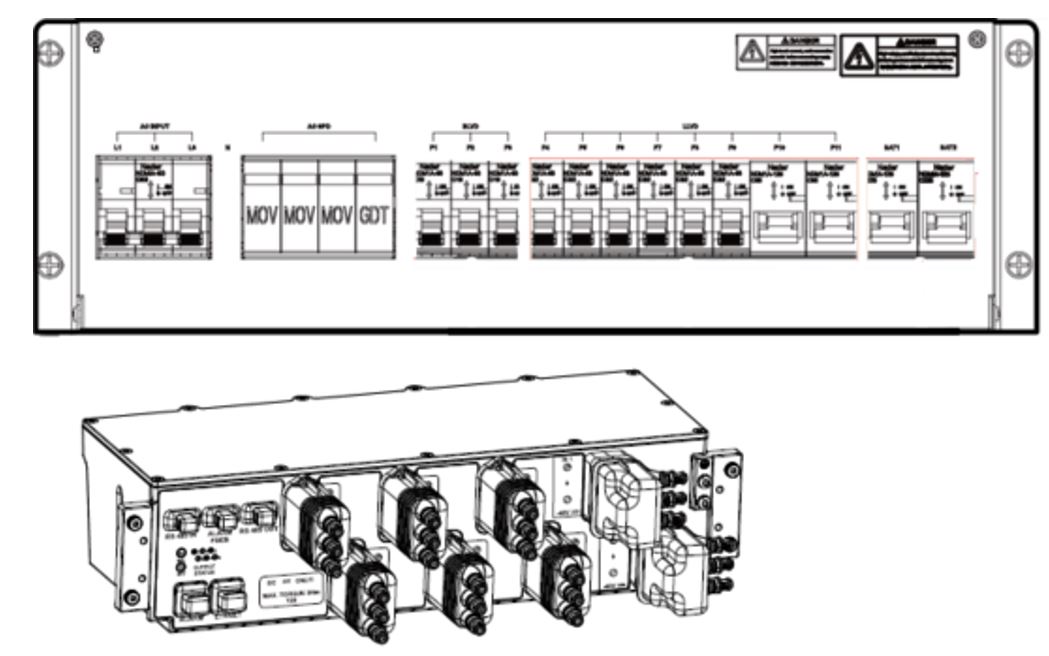
Figure 5 Sample of Power Distribution Units from different vendors
Although the primary distribution system can directly feed loads if desired, a secondary distribution system may be used for larger Scenarios.
- Monitoring and control system. Component that includes alarm collection, processing and metering. Control systems include rectifier float/equalize control and timing, parametric recorders, local area network (LAN), serial port, with modem interfaces. In some solutions it is embedded in the PDU or rectifiers.
In addition to the components above, NaaS Operators may consider a Standby AC Power Source that provides standby power through an engine-generator set fueled by diesel, propane (liquefied petroleum gas, or LPG) or liquefied natural gas. This architecture is shown in Figure 6.
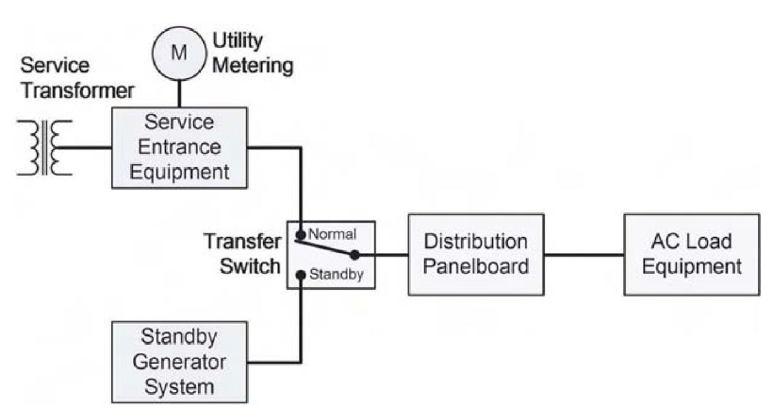
Figure 6 Simplified on-site AC power distribution system with a standby generator.
There are pre assembled Grid Power Systems available for RAN and Transmission equipment used in Low power consumption scenarios. Some vendors offer their DC power system for indoor or outdoor locations embedded in IP65 cabinets including a cooling system. The size of the system is customizable depending on RAN Equipment Power Consumption and Engineering requirements. The Figure 7 below shows a Power system commonly used in rural environments:
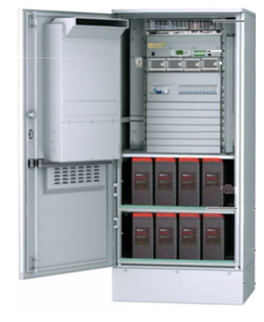
Figure 7 Outdoor DC Power System
2.4 Solar System Overview
Base stations need to provide 24/7 operations. They are not only installed in urban areas, but also widely distributed in various environments such as deserts, islands, mountain tops. They are unattended and have high demands on the reliability and lifespan of power supply.
Many rural locations do not have a grid line that is readily available from the RAN site. As an alternative, the recommended choice is the Solar Power System. Its cheaper than the cost to add utility poles on the RAN site.
In the Solar Power Systems, the energy conversion is static and needs much less maintenance compared to generators relying on physical movements of mechanical parts. It is most suitable for a remote area power supply system when the base station site load is less than 2kW.
However, solar is only produced during the day so energy storage is required for these systems. Energy storage is what makes a solar system more expensive than grid power in rural areas. However, a cost-benefit analysis should be performed by the NaaS Operator to decide between Grid and Solar when both options are available. Table 2 lists the pros and cons of Solar Power Systems.
|
Pros |
Cons |
|
Renewable Energy Source |
Higher CapEx |
|
Reduces Electricity Bills |
Weather Dependent |
|
Low Maintenance Costs |
More Batteries are required |
|
Safer than traditional electric current |
Higher Space Requirements |
Table 2. Advantage and Disadvantages of Solar systems
2.5 Solar System Description
The Solar power system consists of electricity generation, energy storage, energy conversion, and management equipment. Energy generation equipment includes a photovoltaic array. Storage equipment includes a battery pack. Energy conversion and management equipment comprises in Charge controllers with DC converter and in some cases an inverter switch.
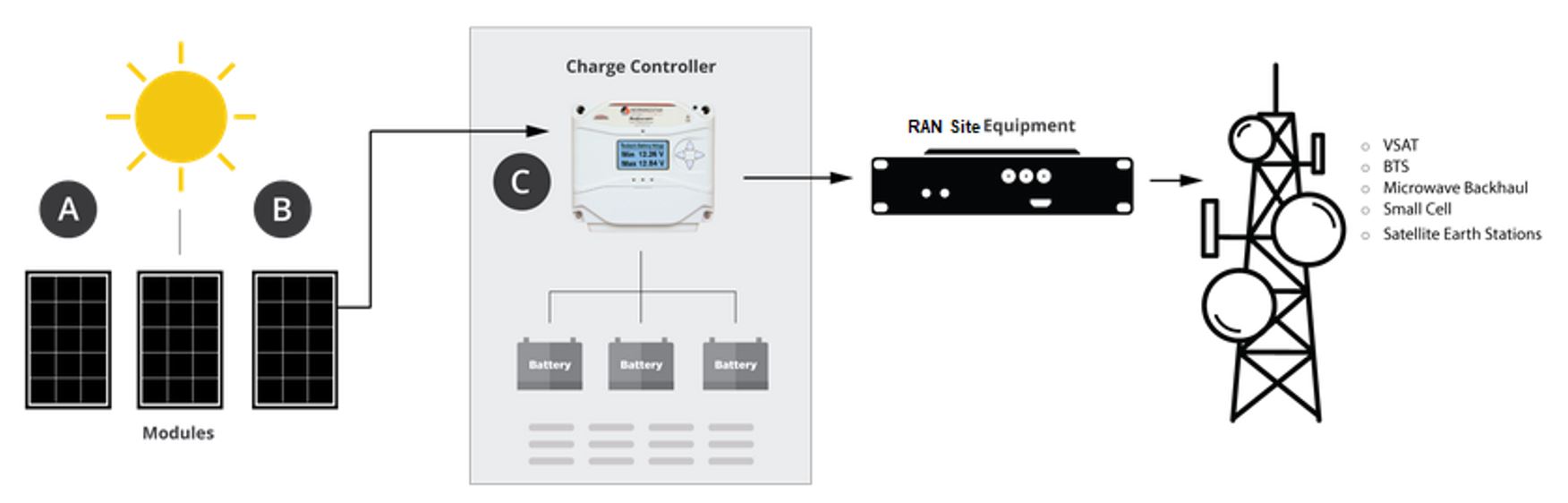
Figure 8 Basic Elements of a Solar Power System
2.6 Site Layout Overview
The Site Layout is an important part of RAN site engineering. Site Layout refers to the technical drawings that show information about power and network equipment at RAN sites.
The Site Layouts are created and used by engineers, builders, field technicians, etc. for the electrical, and RAN systems of different buildings, towers, or data centers. They consist of lines, special symbols, dimensions, and notations used to clearly show the RAN and Transport equipment location and the scheme of electric wiring within.
Site Layout will help installation technicians to locate the equipment within the site facility, including the antennas and RRUs in the tower, which will help to protect the equipment during the installation avoiding damage to the equipment due to wrong installation protecting NaaS operators investments.
This Module suggest the following layouts for the NaaS Operator procedures:
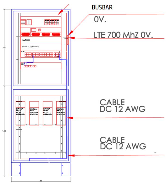
Figure 9 Sample of electrical wiring layout in a cabinet
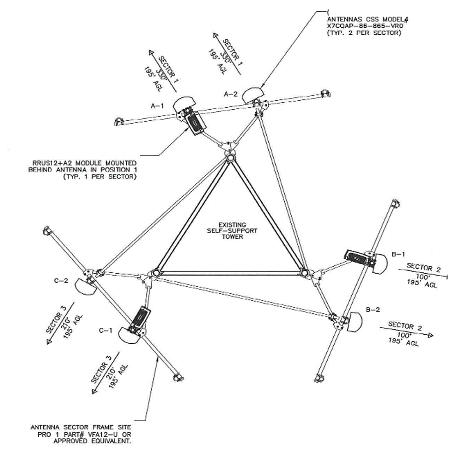
Figure 10 Sample of Antenna System Layout
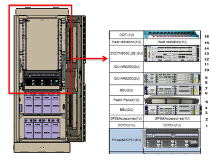
Figure 11 Sample of Cabinet Layout including Power, Transmission and RAN equipment
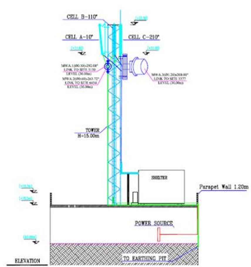
Figure 12. General Site Layout Sample
2.7 Power Connections: Power Over Ethernet
Power over Ethernet is, generally speaking, a technology that allows sending power and data over UTP cables used for data transmission, at a range of up to 100m (333ft). The operating voltage for energy transmission is always under 60V, power is always under 100W, and the power source is protected against short circuits. With that, PoE is safe for people and for equipment. PoEs major advantages over using a local AC power adaptor are:
There are two ways to deploy PoE technology: using a PoE switch, or by installing PoE injectors in the existing networking infrastructure. PoE-capable switches offer the advantage of an integrated solution that requires only one cable for the network connection. PoE injectors are a power source that can be used in combination with a non-PoE Switch.
Use Cases for PoE in Outdoor Small cells
Outdoor cells are located in places without easy access to electricity and have the added disadvantage of requiring IP66 or IP67 weather protection, which means that minimizing the number of input ports is critical. PoE can be used to deliver power, either:
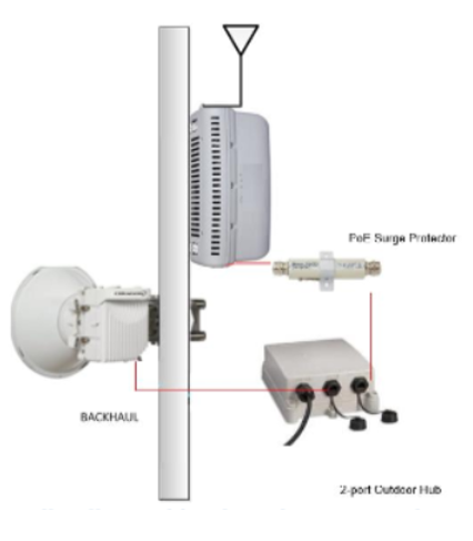
Figure 13 Small Cell + Backhaul Deployment using a PoE HUB
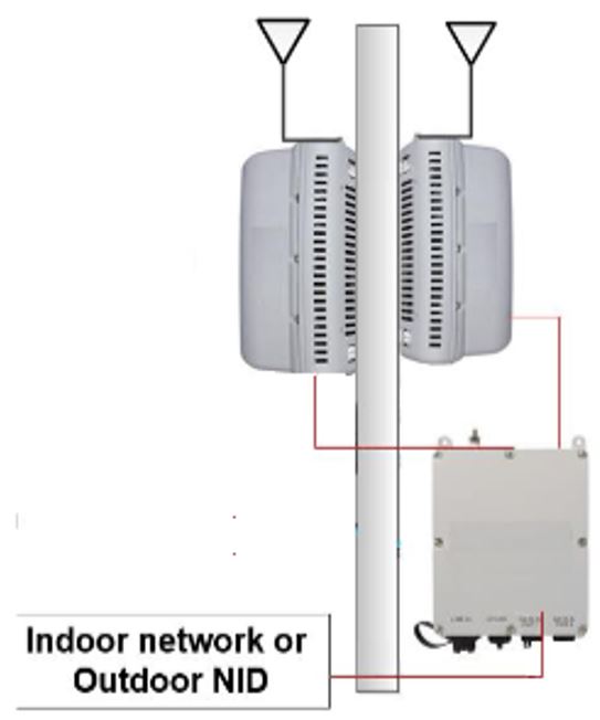
Figure 14 Switch with PoE capabilities feeding 2 small cells
2.8 Electrical Protection
Most of the power systems include mechanisms to protect the power equipment and the connected load of electrical disturbance. The set of recommended protections are listed below:
However not all power system include these protections, Naas operators must be aware of which kind of protection their chosen power system includes, this information can be found in the power equipment datasheet. If it is detected that any of the recommended protection is missing, NaaS Operators should add the missing protection with additional devices as required. Some devices used in RAN sites are shown in Figure 15, and described below:
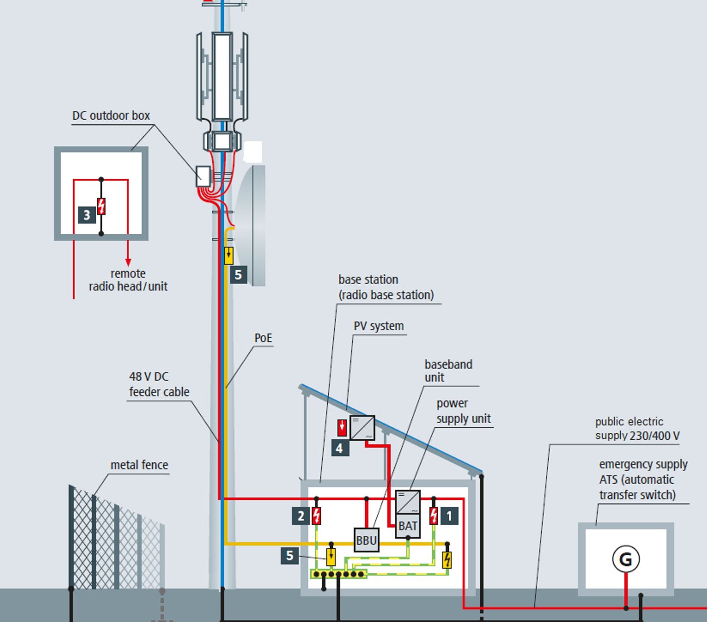
Figure 15 RAN site electrical Protection
3 Power System Design
This section describes guidelines to size and select the basic components of the DC power system that feeds a RAN site. The Sizing and design of AC Power solutions used for external HVAC systems (heating, ventilation, and air conditioning), lights or any other AC equipment at the site is out of the scope of the PlayBook.
3.1 Power System Design Process
A DC power system must provide the specified voltage range and current to the equipment and batteries when the primary power source is available. The batteries must provide reserve power for a certain amount of time giving autonomy from the main source when it fails. The objective of Power System Design is to ensure the power requirements are met with a proper autonomy for each site optimizing the system. As depicted in Figure 3 in Section 2.2 the design process includes calculation of the RAN site power consumption, development of the system requirements and sizing of the system based on those requirements.
New systems are the easiest to design because there are no constraints caused by existing and many times inadequate infrastructure. The new infrastructure is built to accommodate the new systems and is possible to use a wide variety of new equipment. Expansion or retrofit of existing systems, particularly older systems, usually is more difficult because of the physical and electrical limitations.
3.2 Load Calculation
The Load calculation of the RAN site is determined by the power consumption of all the elements of the site, measured in Watts(W), and it is used to properly size the power equipment. Most of the Equipment to be powered at RAN sites consists of:
The DC load caused by transmission equipment such as switches and routers, for practical calculation can be considered constant regardless of traffic, In the same way the power consumption of radio Baseband or Microwave IDU can be considered constant.
In case for in-built cooling system within power cabinets or other cabinets, the vendors mention the power consumption at certain temperature commonly at 25C and is the one used for load calculations.
The load characteristics of the Radio Unit equipment are quite different from switching systems. there is a relatively small fixed (static) load component and a large variable load component. The variable component depends on traffic (each active channel contributes to the load), and daily variations are fairly predictablemidmorning, midafternoon, and evening.
So, the mathematical equation for the power consumption of a RAN site is:
![]()
(Eq. 1)
Where:
The best way to obtain the power consumption of the RAN site elements is from the vendor documentation. Commonly can be found in the equipment datasheet or the environmental product declaration.
Below is an example of a Load Calculation in a Grid AC-DC Power System :
Example: Table 3 is an example of the power consumption in watts of a radio baseband for different configurations:
|
Configuration |
Total Power Consumption (W) |
Total energy consumption (kWh/ year) |
|
1 transport board + 1 capacity board |
160 |
1402 |
Table 3 Example of a Radio Baseband Power Consumption
An example of Radio Units power consumption is showed in Table 4 In this sample the vendor indicates the Radio Unit typical power consumption in Watts for 48VDC input, at 25C, with +/- 10% margin. The average power consumption detailed in Table 4 considers 6h low hour load, 10h medium hour load and 8h busy hour load / 24h.
|
Configuration |
Output Power per carrier (W) |
Power consumption (W), ETSI 202706 average load PRRH, static |
Power consumption (W), ETSI 202706 busy hour load PBH RRH, static |
Power consumption (W), 100% RF power load P100% RRH |
|
1/1/1 4Tx |
4×40 |
879 |
1076 |
1557 |
|
1/1/1 4Tx |
4×20 |
657 |
755 |
965 |
|
1/1/1 2Tx |
2×40 |
540 |
637 |
874 |
|
1/1/1 2Tx |
2×20 |
430 |
479 |
581 |
Table 4 Power Consumption of a Radio Configuration
An example of a Microwave in Split-Mount configuration is showed in Table 5.
|
Microwave Split-Mount Solution |
|
|
Power consumption per carrier |
55W outdoor radio 15W indoor baseband |
Table 5 Power Consumption of Microwave transmission equipment
Table 6 is an example of a Cooling System power consumption embedded within an Outdoor Cabinet in these cooling systems the power consumption varies according to the temperature.
|
Cooling System in Outdoor Cabinet |
|
30 W idle +23C (+73.4F) |
|
50 W typical +55C (+131F) |
|
150 W max. ambient |
|
500 W cold start (heater active) |
Table 6 Outdoor Cabinet Cooling System Power Consumption
Calculate the total power consumption of a RAN site using the power consumption showed in Table 3, Table 6, Table 4 and Table 5 using the following assumptions:
a) A Macro site with 1 baseband and 3 Radio Units in (1/1/1 2Tx) with 20W RF Output Power configuration.
b) Use Microwave transmission in Split-Mount configuration with a single carrier.
c) The deployment location has a max temperature of 25C and a Minimum of 13C constant during all year.
Solution
1. Baseband Load Consumption
In this example it is indicated in Table 3 that the baseband power consumption is 160 W. The Radio Units use a (1/1/1 2Tx) with 20W RF Output Power configuration the safe assumption is to take the average power consumptions (6h low hour load, 10h medium hour load and 8h busy hour load / 24h) adding a 10% margin in this case the Table 5 indicates 430 W(1.1)=473W. The Macro Base-Station consumes a total of 160W +473W=633W.
2. Split-Mount Microwave Transmission Equipment
The DC load caused by this type of equipment is constant regardless of traffic. The sample indicates: 55W for the outdoor radio and 15W for indoor microwave baseband a total of 70 W
3. Cooling System Consumption
In this example it is indicated that the ambient temperature is a maximum of 25C and a Minimum of 13C constant during all year. Table 4 indicates 50 W typical +55C (+131F).
So, from Equation 1:
![]()
(Eq. 1)
= 633W+70W+50W = 753W
3.3 Grid Power System Dimensioning
There are two basic components of the Grid AC-DC Power System that should be sized to feed the DC load: The rectifiers, which converts AC current to usable DC current, and the batteries that assume the load when external power is interrupted. This section includes guidelines to size Rectifiers and Batteries accurately, based on load calculation and the autonomy requirements.
3.3.1 System Operating Voltages and Ranges
To properly size the batteries is required to obtain the Operative Voltage of the RAN site. The equipment with the highest minimum voltage (VME) and lowest maximum voltage (VLM) generally will set the operating range of the power system in a RAN Site.
Example.
All the equipment used in a RAN site has a nominal power of 48VDC. One equipment has a permitted operating voltage of 36.0 to 60.0 VDC. Other equipment operative voltage range of 42 to 56 VDC.
Therefore, the high limit for the power system must be set to 56.0 V even when other equipment in the same site operates satisfactorily at 60VDC. It should be noted that prolonged operation at higher voltages almost always reduces equipment reliability even when the equipment is rated for the higher voltage. The minimum operating voltage is 42V even when there is equipment in the same RAN site that can operate at 36V.
3.3.2 Battery System Design
A battery system consists of a set of industrial batteries with enough power to feed the RAN site, this section will provide guidance to choose a battery technology that suits NaaS operator needs and engineering guidelines to properly size the battery bank that fits the equipment power requirements and provide enough autonomy.
The results of the battery system design are:
3.3.2.1 Battery Technology:
There are two battery technologies used in RAN sites: VRLA and Lithium batteries. A comparison between both is analyzed in Table 7.
|
VRLA |
Lithium ION |
|
|
|
|
Requires More Recharging |
Faster Charging and Discharging |
|
Maintenance at least once a year |
Maintenance at least once a year |
|
Lifespan of 5-7 years |
Lifespan of more than 10 years |
|
Least expensive |
More expensive |

Table 7 VRLA vs- LI-ION
Currently, VRLA batteries are predominantly adopted in RAN sites, however, the use of Li-ion batteries is increasing in commercial deployments. This module will consider VRLA batteries to calculate the bank sizing in the Power system.
3.3.2.2 Battery Bank Capacity
The Battery Bank consists of two main characteristics: the number of batteries and strings. Commonly for a 48 V system a string is an array of 4 x 12V batteries connected in series. Additional arrays increment the autonomy of the system.
The factors used to calculate the required battery capacity in ampere-hours (Ah) consists in the following inputs:
a) Equipment load current in Amperes (A):
The total equipment load can be calculated with the power consumption and nominal voltage of the RAN site:
![]()
(Eq. 2)
b) Autonomy requirements in hours (H):
Autonomy requirements is the reserved time that the battery bank will provide energy to the site in case a power outage from the main power source. The recommended range is between 8 to 12 h reserve time.
c) Battery required capacity (Ah):
To determine the required capacity battery firstly is needed to calculate the battery final voltage (VBF), which is the minimum voltage to which the battery can discharge and still maintain equipment operation. The battery final voltage must be greater than the minimum equipment operating voltage (VME) by an amount equal to the voltage drop from the battery terminals to the equipment terminals and includes all circuit conductors and connections in between(usually considered to be 2.0 V for -48V systems). So VBF is defined by the equation below:
![]()
(Eq. 3)
To calculate the discharge factor is required to calculate the required final cell voltage (VCF) of the batteries defined by :
![]()
(Eq. 4)
Where:
![]() = 24cells for 4 (12V) VRLA batteries in 48V systems
= 24cells for 4 (12V) VRLA batteries in 48V systems
Example If the minimum operating voltage of a RAN system is 38VDC :
![]()
The final cell voltage (VCF) equals the battery final voltage (VBF) divided by the number
of cells (NCell) :
![]()
VRLA batteries used in the RAN sites provide 12 Volts, so for a 48V system, 4 batteries are required to be connected in series. VRLA batteries are built from 6 electric cells, each cell provides 2 Volt (nominal voltage) to the battery system. Battery manufacturers provide their discharge characteristics based on the constant current to the load within a certain period of time until the battery cells reach a final voltage Figure 16 shows a sample of the discharge characteristics of a battery with 12V 91Ah (8Hour/25C) up to final discharge voltage of VCF of 1.75V.
![]()
Figure 16 Sample of constant current discharge data units: (Amperes) at 25C
The required capacity is defined by
|
(Eq. 5) |
![]()
Where:
C= The required Capacity of the Battery Bank in (Ah)
![]() = Nominal Capacity of the battery as is indicated in the vendor documentation (Ah).
= Nominal Capacity of the battery as is indicated in the vendor documentation (Ah).
![]() = Constant Discharge Current during a certain time up to reach a specified VCF (A) .
= Constant Discharge Current during a certain time up to reach a specified VCF (A) .
At= Total Current of the RAN site equipment (A).
Example A RAN Site with minimum equipment voltage of 38V and a power consumption of 753W, requires 10 hours of autonomy. Determine the required capacity of the battery bank taking as a reference the sample of constant current discharge of Figure 16
Solution. From previous examples :
1.-Calculate At From Eq. 2 :
![]()
2.-From the sample of constant current discharge of Figure 16 the available current for 10 hours is 9.5 A the From Eq. 5 :
![]()
3.3.2.3 Number of Batteries and Strings
The arrangement of the batteries in series determines the voltage polarity. Just as the voltage of a battery system is increased by connecting the batteries in series, the ampere-hours and kilowatt capacity of the systems can be increased by connecting strings of series-connected batteries, in parallel.
If each of the 12 V batteries shown in Figure 17 is rated for 91 amp-hours, each series string of batteries could be expected to produce 91 amps of current for one hour.
Capacity is directly related to the size of the battery; but, rather than spending more on larger batteries, it is possible to achieve the same boost to capacity by adding more strings of batteries to the system in parallel as opposed to adding them in series.
This option also provides safeguards against the failure of an individual battery, which would remove its string from the system altogether. By connecting in parallel, the spare capacity is already online and ready to maintain the current for its rated length of time. A diagram of a parallel battery strings rated at 182 amp-hours is showed in Figure 17. Note that, if a battery failed in any of the two series strings, the remaining string would continue to supply steady power at 91 amp-hours as indicated in Figure 17.
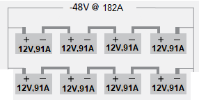
Figure 17 VRLA multi-string battery configuration offering additional redundancy
After calculating the total battery capacity, it is necessary to determine the number of battery strings. As a general rule, the number of battery strings should be the minimum necessary.
If the total required battery system capacity is to be divided equally across two or more strings, the required number of strings is determined from:
|
(Eq. 6) |
![]()
where
![]() = number of battery strings in parallel
= number of battery strings in parallel
![]() = individual battery string capacity (AH)
= individual battery string capacity (AH)
![]() = The required Capacity of the Battery Bank in (AH)
= The required Capacity of the Battery Bank in (AH)
There is no technical limit on the number of battery strings that may be connected in parallel but there are practical limits. As a general rule, the battery manufacturer should be contacted if more than five strings are to be paralleled. Some manufacturers do not recommend more than four or five parallel strings.
The widget $$link widget$$power system sizing contain a tool to size the battery bank for a RAN site will help NaaS Operators to calculate the required capacity of the battery bank and a recommended Battery Array.
3.3.3 Rectifier System Design
The rectifier system capacity must be large enough to not only operate the load equipment but simultaneously recharge the batteries at the desired time. Rectifiers used in telecommunications applications consist of modular rectifiers commonly equipped for N + 1 redundancy, operated in parallel, and almost always set up for load sharing.
With modular rectifiers, it is relatively simple to adjust the capacity by unplugging unneeded rectifier modules or using modern controllers that can be programmed to activate only the necessary rectifiers. The controllers on some rectifier systems can be set up to automatically shut down unneeded rectifiers during float operation and to bring them back online when needed for battery recharge. For RAN site applications there is several options for rectifiers, commonly are embedded with the power controller in 1 Rack Unit, Figure 18 shows a rectifier modular system with 2 rectifiers.

Figure 18 Common Rectifier Modular System for RAN sites
There is Two considerations to decide the rectifiers system:
1.-Input Power: Switch mode rectifiers are the preferred choice RAN sites since they can support multiple AC inputs and have a broader operating rangefrom single-phase to three-phase inputs. This flexibility means fewer rectifiers are requiredsaving money, space and maintenance.
2.-Output Power: The output power of rectifiers for RAN sites are available in a wide range commonly from 110W to 4.4kw. There is no technical limit to the number of rectifiers, but a simple economic analysis may reveal that a small number of large rectifiers is cheaper than a large number of small rectifiers.
The Rectifier system design requires the selection of
● Capacity
● Quantity
3.3.3.1 Capacity and quantity of rectifiers
Even the smallest system will have at least two rectifiersone to carry the load and recharge the battery and another configured for hot-standby operation.
Industry baseline requirements specify that the rectifier system should be designed to recharge a fully discharged battery to 95% of its nameplate capacity rating within at least 24 h while simultaneously operating all load equipment. This requirement should be met when the equipment is operating at its busy hour load (normal condition).
The total normal condition load current is one parameter used to calculate the required rectifier system capacity. Note that normal condition load current is used here instead of peak.
The rectifier system capacity is calculated from:
|
(Eq. 8) |
![]()
Where
● tRecharge = battery recharge time (h)
● Cnom= battery nameplate capacity at 25C and 8-h rate to 1.75 V/cell (Ah)
● IRS = rectifier system capacity with N rectifiers (A)
● IEQ = normal condition equipment load current (A)
● FBatLoss = battery loss factor (typically 1.10 to 1.15 for VRLA batteries)
Where modular rectifiers are to be used, the total number of modular rectifiers (NRM) is determined from the rectifier module current rating (IRM) from:
|
(Eq. 9) |
![]()
rounded up to the next higher integer value. This assumes that all rectifier modules have the same rating, which would be true in new installations and replacements. Where additional rectifier capacity is added to an existing installation, the redundant rectifier (or rectifiers) must be at least as large as the largest rectifier in the system. For example, if an installation has two 50-A and one 100-A rectifiers for the load and battery recharge, redundancy would be provided by adding a second 100-A rectifier or two additional 50-A rectifiers. This protects the system from the failure of any rectifier in the system
Example:
A battery system of 182Ah is used in a system where the equipment load current is 15.68 A. Determine the total rectifier system capacity and number of rectifier modules if each module is rated 50A.
Solution
From (Eq. 8)
![]()
From (Eq. 9)
![]()
As a result, for this vendor, the required Rectifiers Sum Up 2 Rectifier of 50A with a redundancy configuration (N+1)
The widget $$link widget$$power system sizing contain a tool to size the rectifiers for a RAN site based on the content on this section
3.4 Solar Power System Design
This section outlines the main features of a typical remote-area, stand-alone, all-DC Photo Voltaic-powered system with reference to design features, installation, and sizing.
Defining the system load is the first step to Solar Power System Design. Method in Section 3.2 shows the general methodology to calculate the load of a RAN site suitable for any power system.
The total load of the RAN site along with the average solar irradiation and PV Panels efficiency is used to size the Photo Voltaic Panels array which must be capable of producing power to supply the load current for 24 hr/day and to supply the battery charging current for the daily peak sun hours at the site location.
The sizing of the battery bank is different from the Grid power system since the autonomy requirements for a solar power system are greater and are estimated in days. The size and cost of a Solar system is proportional to the energy consumed by the load. Reducing the electrical load by selecting energy-efficient equipment will result in a corresponding reduction in the system cost.
Figure 19 shows the design process for a Solar Power System:

Figure 19 Solar Power System Design Process
3.4.1 Sizing Photo Voltaic (PV) Panels
In order to size the PV panels required to power a RAN site is required to know the Nominal Power of the PV Panel. The maximum electric or nominal power of the PV panel can be defined as its Peak Power (in Watt Peak). The Peak Power of solar panels is registered under the following Standard Test Conditions:
● a light intensity of 1.000 W/m
● sunlight hitting the positioned solar cells perpendicularly
● a temperature of 25C at the solar cells
The Nominal Power is a specific feature of the PV panel, regardless of the location where it is tested. Under these standard conditions, the nominal power of solar panels can be compared with each other. A solar panel with a Peak Power of 5 kW in Peru is for example exactly the same as such a panel in the USA.
The real electric power of the PV panels is primarily dependent on the number of hours of sunshine to which they are exposed. Sun hours vary greatly depending on the site location and local climate. To determine the average solar Irradiation go to $$link$$https://globalsolaratlas.info/map. Figure 20 shows the global horizontal irradiation pattern

Figure 20 Global Horizontal Irradiation Map
The number of solar panels depends on the average solar irradiation in the place of interest and nominal power (Pnom) of the solar cells. The nominal power is obtained assuming that solar irradiation is 1000 W/m2. Equation 10 shows the expression to calculate the number of solar panels:
|
(Eq. 10) |
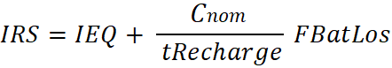
Where
● TDLoad is the daily total energy required by the systems in Wh,
● Ƞg denotes the losses due to the inefficiency of the solar cells (around 10%)
● Fc is a correction factor (Fc=1.3) introduced as the solar cells have to generate energy for the system and for the batteries that are accumulating the energy.
● Gdm is taken as the average daily solar irradiation during the worst month of the year (for example in the Loreto region in Peru, the solar radiation is 4270 Wh/m2).
Example: Size the Solar Panels for a solar system if batteries and panels have the following specifications:
Solar cell: Solar World (Pnom = 300 W per panel)
Consider the same load as the one in the example of section 3.2
Consider the solar radiation of the Loreto region in Peru
Solution:
The number of solar panels and batteries will be obtained from equations (10)
Solar Panel Calculation:
TDLoad of RAN Site equipment = 753Wh X 24h = 18,072Wh
Pnom = 300W
Gdm = 4270 Wh/m2
PV Solar Cell Inefficiency Ƞg = 10%
Solar Cell correction factor fc = 1.3
![]() =
= ![]()
![]()
The widget $$link widget$$power system sizing contains a tool to size the solar panel for a RAN site based on the content on this section.
3.4.2 Battery Bank Capacity Estimation
The methodology to used in Section 3.3.2 uses the Discharge capability of batteries, vendor expresses it by the 20-hour rate. The autonomy requirements for a solar power system are greater and are estimated in days therefore is required another method.
The capacity of the batteries (in Wh) should be enough to provide electrical energy to the system to be up to ![]() without any charging procedure. For VRLA batteries the capacity must satisfy:
without any charging procedure. For VRLA batteries the capacity must satisfy:
|
(Eq. 11) |
![]()
where
● ![]() Is the capacity required of the battery bank (Wh)
Is the capacity required of the battery bank (Wh)
● TDLoad is the daily total energy required by the systems in Wh,
● Ƞg denotes the losses due to the inefficiency of the solar cells (around 10%)
● Pdmax = A parameter to impose that a battery should have at least 20% of its maximum capacity (Pdmax =0.8).
Batteries sizing Calculate the required capacity for a Battery Bank used in a solar system with the following parameters
Assume Ndays = 1 days of autonomy without any battery charging, as the worst case.
Consider the same load as the one in the example of section 3.2
Solution
The required capacity will be obtained from equation (11).
From section 3.2 TDLoad 753Wh X 24h = 18,072Wh
![]()
The widget $$link widget$$power system sizing contains a tool to calculate the required capacity for a Solar Power System Battery Bank, please note that after calculating the required capacity, the battery bank should be designed accordingly, the Section 3.3.2.3 indicates the required batteries and strings needed.
3.4.3 Design Considerations, Panel Array: Position and Tilt
If the RAN site deployment location is in the north of the equator, the sun leans south as the Earth orbits. Facing the PV array to the south will capture the most daylight and produce more energy. However, if the RAN site deployment location its the south of the equator, it would be more efficient to face the PV array to the North.

Figure 21 The relationship between the sun and earth. The declination angle (δ), the latitude (ϕ), and the solar time angle (t) are also shown on it.
Tilt from horizontal is required to achieve a better angle at the sun and help keep the solar modules clean by shedding rain or snow. The optimal tilt angle is the latitude 15. In summer months, the optimal tilt angle is usually 15 less than the latitude, whilst in winter months; it is 15 more than the latitude.
Additionally, NaaS Operator may consider the following guidelines to mount the PV array:
● PV modules are very sensitive to shading; once a solar cell or a portion of a cell is shaded, it becomes a load and draws power instead of producing it. Thus, PV modules should never be shaded by nearby trees or structures.
● Temperature at the back of the modules can rise to 80C if they are poorly ventilated. Installing the solar array in an area with natural ventilation will improve system performance and extend its life.
● The mounting option must allow for safe maintenance and possible replacement of individual modules.
4 Core Site Layout
Core Site Layout consists of the design considerations of the room and the layout of the Core equipment in the Room and the rack.
A Core site layout has two components: the structural layout of the empty room which may be obtained from the site engineering in the form of blueprints and the equipment layout of what will go in the room. Note that in the case where NaaS Operators decide to lease a space in a data center, the room is pre-existing, and the only option is to layout the equipment in their cabinet.
The equipment layout shows the footprint of IT equipment and the footprint of power and cooling equipment. In order to protect the IT equipment from overheating the layout should consider an airflow path. The following subsections provide guidelines to layout the rack in a room considering the airflow of the equipment, the equipment layout within the rack as well as key considerations for the cabling layout.
4.1 Control of airflow using hot-aisle/cold-aisle rack layout
The use of the hot-aisle/cold-aisle rack layout method is well known and commonly used in a data room layout. The basic principle is to maximize the separation between IT equipment exhaust air and intake air by establishing cold aisles where only equipment intakes are present and establishing hot aisles where only equipment hot exhaust air is present. The goal is to reduce the amount of hot exhaust air that is drawn into the equipment air intakes. The basic hot-aisle/cold-aisle concept is shown in Figure 17.
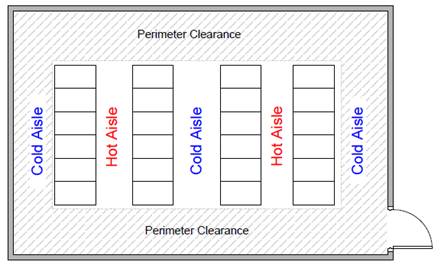
Figure 17. Basic hot-aisle/cold-aisle layout plan
In Figure 17, the rows represent the IT equipment enclosures (racks). The racks are arranged such that the adjacent rows face back to back, forming the hot aisles. The benefits of the hot-aisle/cold-aisle arrangement become dramatic as the power density increases. When compared to random arrangements or arrangements where racks are all lined up in the same direction, the hot-aisle/cold-aisle approach allows for a power density increase up to 100% or more, without hot spots, Decreasing greatly the power consumption of the cooling system.
4.2 Server Rack Layout
In terms of layout, rack density should be considered. The more free-space within a server rack, the greater the room for airflow. Vertical space can be left between servers and IT devices to help cooling. Heat sensitive devices, including UPS batteries, can be placed towards the bottom of a server rack. Heavier devices are also best placed towards the bottom of a rack.
Hardware should ideally be logically grouped for ease of management and access to sockets, outlets and ports, whether for power or networking. Ideally within the middle to higher-level area of the rack.
Some manufacturers have an online free to use tool to elaborate a rack layout with their products and generic boxes, NaaS operators may consider this option to organize their rack layouts, additionally, there are several free web-based tools to elaborate a rack layout some others has to be purchased but have additional features that consider ventilation and PDUs.
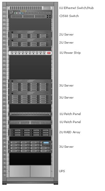
Figure 18. Rack Layout
NaaS Operators may use an asset list for each device within a server rack including each model SKU and serial number. These three pieces of information along with a description, date of installation and service dates can be recorded onto a rack management spreadsheet.
Other additional columns recommended include power draw and heat dissipation or efficiency, UPS (uninterruptible power supply) and PDU (power distribution unit) connections. The document is then maintained when equipment is added or removed and/or maintained. The spreadsheet should cover the entire server room installation and each rack or cabinet within it.
NaaS Operators may use the Rack Management spreadsheet to organize their assets and their port connections.
4.3 Layer 1 and Layer 2 diagram
The Core layout design considers the High-level & Low-level design, this subsection considers some of the outcomes of previous phases to create the physical interconnection
A Layer 1 diagram shows the physical connections between the critical pieces of network infrastructure. It includes link speeds and cabling types. Additionally, show individual port numbers or designations. Some considerations to elaborate a Layer 1 & Layer 2 diagram are listed below:
The required VLAN numbers and port connections are indicated in the Core LLD the purpose of L1 and L2 diagram is to map the physical ports with the logical design.
Figure 19 illustrates the L1 & L2 Diagram:
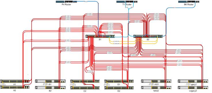
Figure 19. Layer 1 & Layer 2 diagram
NaaS Operators may consider the tools depicted in Table 5 to create an L1& L2 diagram:
|
Tool |
Top Features |
Description |
||
|
CADE |
Free Tool |
Multiple export formats |
Support for multiple diagrams |
Free network design tool with predefined blocks and multiple export formats |
|
DIA |
Free Tool |
Large library of objects |
Open Source |
Simple open-source programmed with a large library of objects |
|
Visio |
AutoCAD support |
Automatic chart generator |
Support community |
Highly flexible popular network design with support from multiple communities and AutoCAD tech support |
|
EDraw |
15-days trial |
Multiple export formats |
Web Version |
All in one application for rack and floor layout include L1&L2 Diagrams |
Table 5. Network Design Tools that include physical connections
4.4 Cabling Layout
The lack of organization can lead to accidental disruption of service. An organized rack decreases human errors, increases efficiency, and improves equipment protection by increasing effective airflow. By using the correct cable management accessories to organize, route and remove unnecessary stress on the cables, data integrity is ensured.
Racks and enclosures can become disorganized quickly if cable management does not remain an ongoing priority. The Core site is a critical point of interconnection, NaaS operators may consider following recommendations to organize and document their connections to ensure optimal performance in the critical equipment, as detailed in the subsections below.
4.4.1 Using Color to Identify Cables
Color provides quick visual identification. Color-coding simplifies management and can save time when its required to trace cables. Color coding can be applied to ports on a patch panel. Patch panels come with different color jacks or have colored inserts surrounding the jack. Cables are available in many colors (The color palette depends on the cable manufacturer). Figure 20 shows an initial recommendation of colors to identify the role/function of a cable type of connection.
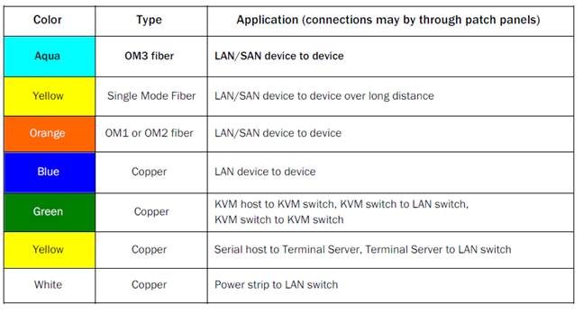
Figure 20. Color Scheme for patch cables
4.4.2 Horizontal Cable Management
Horizontal cable management allows a neat and proper routing of the patch cables from equipment in racks and protect the cables from damage. These cable managers take up the space in racks, so a careful balance between cable manager height and cable density supported is important. 1U and 2U horizontal cable managers are the most common varieties. The density supported varies with the depth of the manager. When choosing cable managers, the NaaS Operator must ensure that the cable bend radius is properly accommodated.
Please note that proper planning should allow a 30% space in the cable managers for future growth.
Figure 21 shows 2 switches using horizontal cable managers.
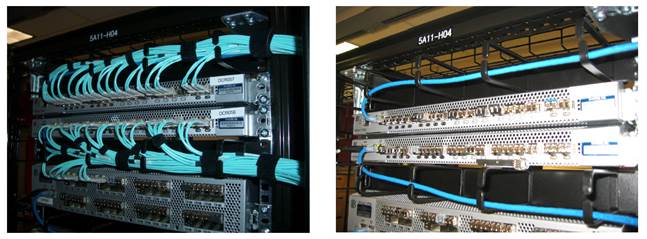
Figure 21. Horizontal Cable Management
4.4.3 Vertical cable managers
For vertical cable managers, there should be additional space required to manage the slack from patch cords and ensure that they can easily route the largest cable diameter. The most convenient cable managers available in the market have hinged doors on both sides of the manager for pivoting the door from either side and allow a complete removal of the door for unobstructed access. A best practice is to allow for 50% for the growth of cables when planning the width. Figure 22 shows three racks using vertical cable managers
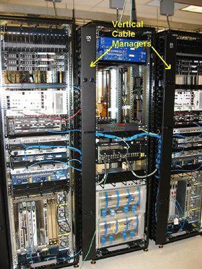
Figure 22. Vertical Cable Management
4.4.4 Overhead Cable Pathways
Overhead cable pathways or trays allow placement of additional cables for interconnecting devices between racks. In order to select the Overhead cable pathways, it must be considered the cable bend radius, weight allowance, aging points for cables and flexibility in installing the pathways. In addition, ensure that pathways allow cable drop points where needed. Figure 23 show overhead cable pathways routing different types of cables.
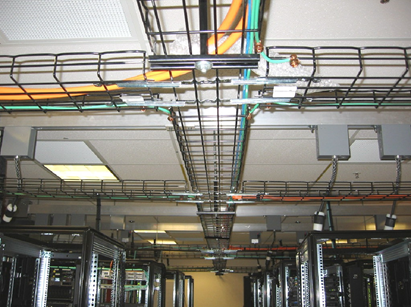
Figure 23. Overhead Cable Pathways
4.4.5 Documentation
The documentation is perhaps the most critical task for cable management. A best practice is to keep the information easily accessible to data center staff on a share drive or internet web service. Naas Operators must assign updates to one or more staff members and make sure it is part of their job assignment to keep the documentation up to date. Furthermore, NaaS Operators may consider creating a training guide, which documents guidelines for installing new cables, cable management components and routing cables. A port mapping spreadsheet is useful for keeping track of used/available ports on the network equipment. It must include the remote device to which each port is connected. NaaS Operators may consider using the Network documentation spreadsheet to document their equipment, cable mapping, and IPV4 usage.
1. Mobile Core HLD Introduction
The Mobile Core High-Level Design (HLD) defines the Evolved Packet Core (EPC) deployment model, features and functionalities which the entire network has to meet. Since the EPC is a centralized element it has a major impact on the entire network performance. Therefore, a precise HLD will provide economic insights on the most suitable deployment approach and plan.
Its important to mention that based on the overall strategy, business case and agreements with Multiple Network Operators (MNOs), not all NaaS Operators will deploy a Mobile Core. Thus, this module applies only to initiatives that require a Mobile Core. More details can be found on the Mobile Core Architecture Module.
The Mobile Core HLD module provides the NaaS Operator background information and methodologies to elaborate a High-Level Design for the Mobile Core Network. It provides guidelines on how to design the mobile core network that interconnects with the Radio Access Network (RAN) to offer security, signaling, authentication and access to end user services.
NaaS Operators span a range of sizes, geographies, and network architectures. That is, there is no one size fits all methodology. For this reason, a generic end-to-end process flow to perform the Mobile Core HLD is presented along with proper guidelines to be tailored to match NaaS Operators requirements and constraints.
The main output of the module is the Mobile Core HLD Design, which includes the Interconnection Assessment, Capacity Planning, and Requirements for Virtual Network Function (VNF) entities, Redundancy Assessment and Bill of Quantities Generation.
1.1 Module Objectives
This module will enable a NaaS Operator to stand-up, run and manage a Mobile Core HLD initiative. The specific objectives of this module are to:
- Provide an information base and fundamentals to perform the tasks associated with Mobile Core HLD.
- Provide detailed how-to instruction on the key HLD engineering tasks.
- Provide an overview of the end-to-end Mobile Core HLD process with instructions for tailoring to specific NaaS environments.
- Provide guidelines to develop a formal Mobile Core HLD recommendation.
1.2 Module Framework
The Module Framework in Figure 1 describes the structure, interactions, and dependencies among different NaaS operator areas.
Strategic Plan & Scope and High-Level Network Architecture drive the strategic decisions to forthcoming phases. Network Design is the first step into implementation strategy which is supported by Supply Chain Management.
The Mobile Core HLD module is included within the Network Design Area and has a direct relation with Transport and RAN HLDs. The generated output of this module will serve as a required input for the Mobile Core LLD module.
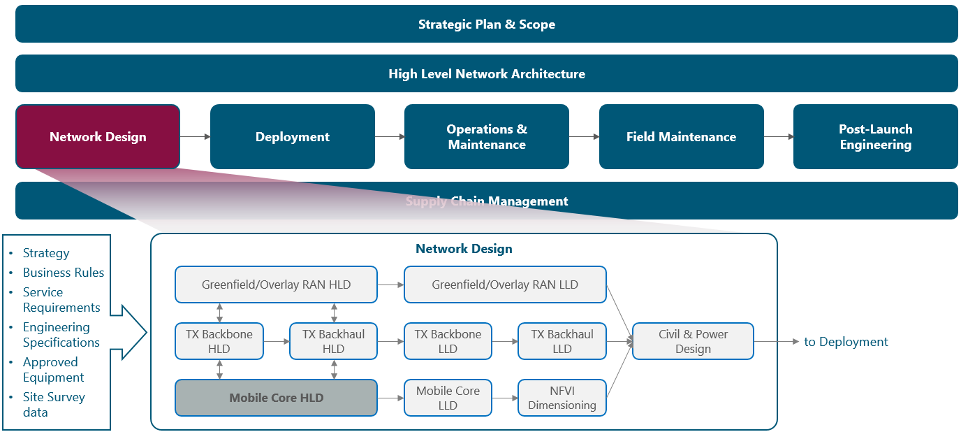
Figure 1 Module Framework.
Figure 2 presents the Mobile Core HLD functional view, where the main functional components are exhibited. Critical module inputs are further described and examined in Section 2.3. In addition, guidance and methodologies to execute the tasks included within each function are described in Section 3.
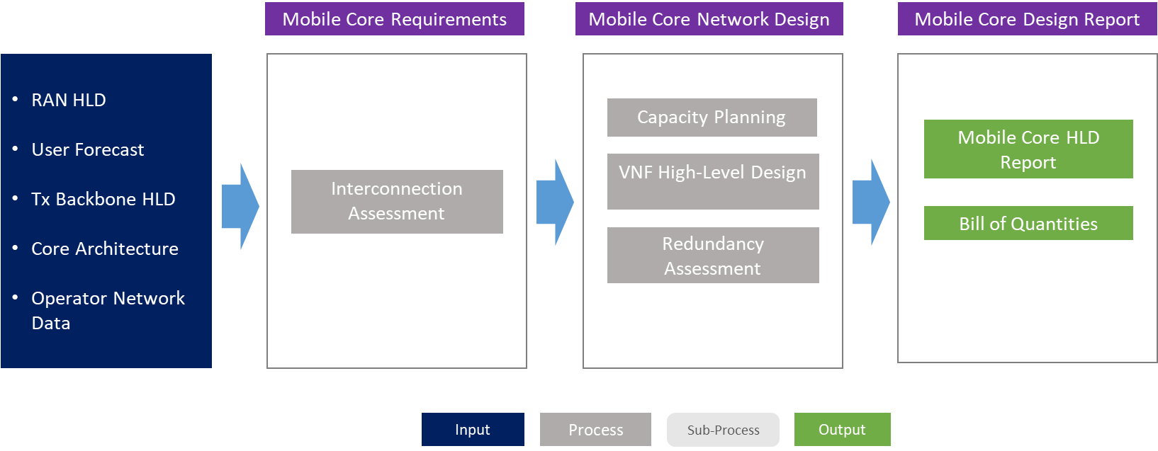
Figure 2 Module Functional View.
The remainder of the module is divided into four sections. Section 2 is a birds-eye view of the Mobile Core fundamentals involved in its design. Once fundamental knowledge is acquired, Section 3 focuses on showing a hands-on view of the tasks involved in the design. Section 4 organizes functional tasks on an end-to-end process flow that can be used as-is or be adapted by NaaS operators to match with their particular conditions. Finally, Section 5 illustrates how to integrate previous elements into a comprehensive High-level Design (HLD) recommendation.
2 HLD Fundamentals
This section presents a general overview of the baseline concepts to develop a Mobile Core Network Design.
2.1 EPC Overview
There are a variety of scenarios when designing a Mobile Core Network depending on the preexisting conditions and the target of the NaaS Operator. The most predominant decision is whether to deploy Mobile Core Infrastructure which is addressed by the Mobile Core Architecture Module. For NaaS Operators deploying an Evolved Packet Core (EPC), the Mobile Core Architecture Module provides a guide to define the logical topology, necessary network elements, interconnection requirements, and virtualized architecture requirements.
Figure 3 depicts the typical EPC Architecture showing the Mobility Management Entity (MME), Serving and Packet Data Network (PDN) Gateways (SGW & PGW), the Home Subscriber Server (HSS) and the Policy and Charging Rules Function (PCRF). Furthermore, it also depicts the interconnection to the RAN network and IP Networks (e.g. Internet)
Connections to external networks are required to offer services to other MNOs that share the RAN network. The number of these connections will depend on the roaming agreements & defined interconnection approach, voice solution requirements, existing Packet Switched (PS) infrastructure and Multiple Network Operator (MNO) strategy.
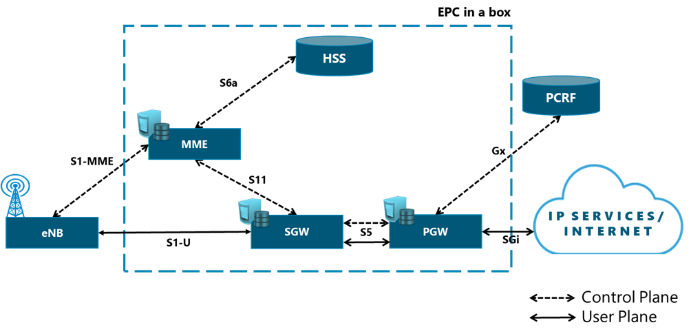
Figure 3 Evolved Packet Core Basic Architecture.
The Mobile Core Architecture Module. provides the overall EPC logical topology and the strategy and requirements for interconnection with other networks (existing 2G/3G infrastructure, customer MNOs, Internet). From these inputs, the Mobile Core HLD Module defines the minimum requirements for the EPC related to Capacity Planning, VNF specifications, the networking protocols architecture and the redundancy mechanisms to appropriately assess available solutions in the market.
2.2 Mobile Core Environment
This section addresses the topics that require attention when developing a Mobile Core High-Level Design.
2.2.1 Multiple Mobile Network Operator (MNO) Design
The NaaS Operator business model requires that multiple Mobile Network Operator (MNO) share the same RAN equipment as seen in Figure 4. Different approaches and solutions to address this issue are available and the choice will depend on the agreement with the customer/partner MNOs.
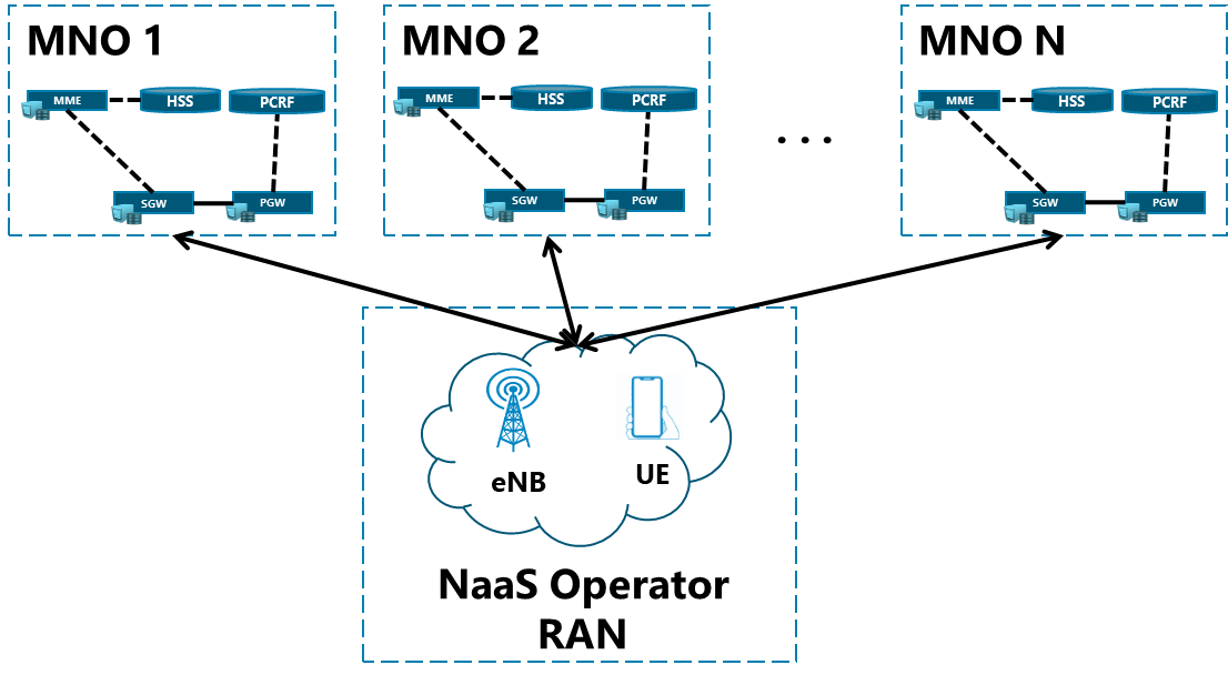
Figure 4 Multiple MNOs sharing the same NaaS Operator RAN.
As discussed in the Mobile Core Architecture Module, the first approach is when the NaaS Operator only implements an MME and SGW entities to minimize the investment, but still getting the control of the RAN. The MME and SGW are shared between operators while user databases (HSS), policy and authentication entities (e.g. PCRF, OCS, OFCS) will remain independent across operators, as seen in Figure 5.
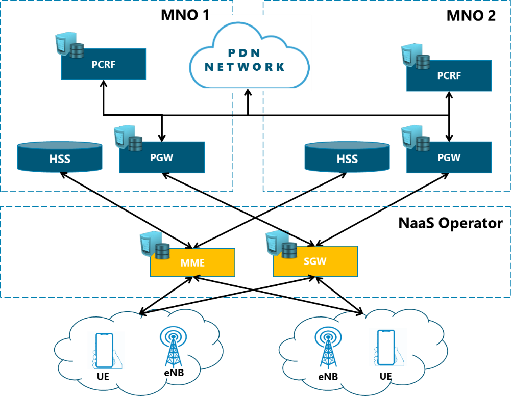
Figure 5 MME-SGW Deployment.
The second strategy consists in deploying all the EPC and PCC elements in a centralized manner as seen in Figure 6. This will allow the NaaS Operator to broaden its market by providing services to MNOs and all types of MVNOs.
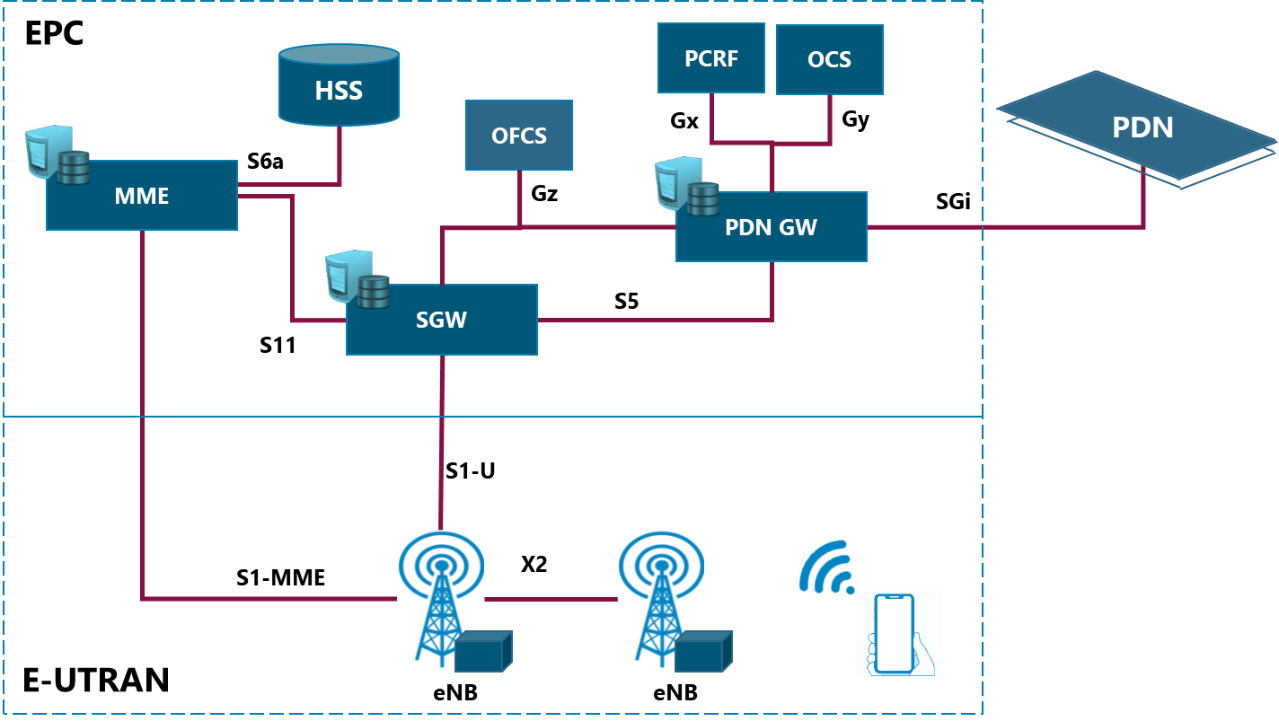
Figure 6 Full deployment of centralized EPC
Finally, in addition to the full EPC deployment, a roaming strategy for interconnection with multiple operators needs to be defined. Guidelines and necessary details to define this strategy are provided in the Mobile Core Architecture Module.
From the HLD point of view, these architectural options impact the Interconnection Assessment and Capacity Planning. For Interconnection, the choice of architecture impacts the number of external connections and protocols to be used on roaming interfaces), while for Capacity Planning it drives the traffic and users dimensioning based on the roaming agreements
2.2.2 Interconnection and Networking Considerations
The Architecture module defines the approach to interconnect to other networks, however, the Interconnection and Networking mechanisms must be defined as part of the HLD. These mechanisms are directly impacted by the number of customer MNOs using the NaaS Operator network to provide service.
Based on roaming agreements and strategy contained in the Architecture module, the number of connections to external MNOs (partners and customers) can be determined, as well as the expected number of roaming users and the number of logical interfaces to match the required strategy.
The number of MNO partners will drive the number of Mobile Core interconnections required, consequently impacting the HLD design. Furthermore, for the virtualized scenario, the networking solution must take into account capacity requirements and the number of logical interfaces to/from all the MNOs using the shared RAN. Even the choice of networking protocols will be influenced by the number of interconnections to external networks as described in section 3.1.
2.2.3 Capacity Planning and Forecasting Estimation Challenges
RAN and Tx HLDs provide the subscriber and throughput forecast for Capacity Planning. In the Mobile Core HLD, the challenges consist of estimating capacity requirements for core elements and interface dimensioning based on the inputs from RAN and TX HLD.
The metrics to be taken into account are:
Additionally, each external interface will have an expected number of subscribers corresponding to all the MNOs sharing the RAN network. The throughput of each external interface is calculated considering its number of roaming subscribers, the type of signaling and the traffic model of those subscribers. The total number of roaming subscribers will also affect the subscriber connection quantity and the signaling load within the NaaS Operator EPC.
2.3 Mobile Core HLD Inputs Description
There is a wide variety of options involved in the mobile core design, so to narrow them, some inputs have to be defined at the beginning of the design process. Identifying the most important inputs and how these inputs impact the overall process is a key step towards an optimized Mobile Core HLD.
The following table contains the most important inputs to develop the Mobile Core High Level Design:
|
Description |
Impact |
Source |
|
|
Mobile Core Architecture |
Architecture of the overall Mobile Core Solution, Service Definition and its required Network Elements. |
Architecture will drive the overall HLD. |
|
|
Roaming Strategy |
Roaming agreements with other MNOs and its approach to interconnection (Local breakout or Home routed). |
It will impact on the Equipment and Interface Capacity. |
|
|
Interconnection Requirements |
Requirements and approach for interconnection to other MNOs and to existing 2G/3G core infrastructure. |
Interconnection Assessment and Capacity Planning are tightly related to the existing infrastructure. |
Mobile Core Architecture Module, Existing Operator Data |
|
High Availability Mechanisms |
Mechanisms to assure the Service Level Agreement, defined as part of the architecture. |
Redundancy techniques are based on this premise. |
|
|
Operator Network Data |
Information related to existing infrastructure (Transport, RAN, Mobile Core). |
Accurate information of existing networks will help Interconnection and Networking Considerations as well as Capacity Planning. |
Operator Network Data, Existing Operator Network |
|
Transmission HLD |
Document containing a high-level view of the transport solution. |
Interconnection and Networking Considerations are based on transport information. |
|
|
RAN HLD |
Document containing a high-level view of the RAN solution, including the expected and forecasted users. |
Capacity planning and forecast are based on user information. |
Table 1 Inputs for the Mobile Core HLD Module
2.4 EPC Core Networking
The interfaces within the EPC and to external networks use a combination of Layer 2 (L2), Layer 3 (L3) and upper-layer protocols to communicate. Many of the EPC interfaces have specific protocol requirements; however, for other interfaces, the NaaS Operator must select the protocols to be used as part of the HLD. The following sections contain a quick overview of L2 & L3 protocols.
2.4.1 Layer 2 Interworking: Ethernet Switching
Layer 2 switching is the easiest way to provide connectivity in a network and it is used to connect all the servers in a virtualized environment. This mechanism will enable NaaS operators to build networks whose hosts can communicate with each other within the same physical network. However, the NaaS Operator may need to separate certain elements or type of traffic which can be done through VLANs
Virtual Local Area Networks (VLAN) are switched networks that are logically segmented on a functional basis, instead of an actual physical basis. It is used extensively in order to deploy logically independent Ethernet networks over the same Ethernet infrastructure. For example, members of the same Ethernet network should be able to communicate with each other. If the switch implements VLANs, the devices within the network can be segmented and separated logically so the communication only happens between members of the same logical network. Further guidance for VLAN design is provided in section 3.1.1.
2.4.2 Layer 3 Interworking: Dynamic Routing Mechanisms
Routing is needed for the NaaS operator to support inter-VLAN communication and to connect to other network domains such as external networks or the Internet. If we take the previous VLAN example, we would be able to communicate between logical networks (VLANs) by adding a router to the Ethernet infrastructure and configure it with a routing mechanism. It is important to note that the VLAN intercommunication can be selectively done. For the EPC implementation, we can administratively communicate two or more logical interfaces by enabling the communication on the router side (e.g. all O&M interfaces across different network segments).
There are two types of routing mechanisms: static and dynamic. Static routing refers that the routing information does not change and it is configured and updated manually on each equipment. Static routes are only used when managing one or two routes and no changes in the network are expected. On the other hand, dynamic routing refers to the routing information being updated automatically on each equipment according to the network changes (e.g. new connections) and conditions (e.g. delay, throughput). It is strongly recommended to always implement dynamic routing because it eases the management and adapts to network growth.
In the following review, only dynamic routing is revised due to the aforementioned capabilities. Figure 7, shows the different classification of dynamic routing protocols, which is reviewed in the section below.
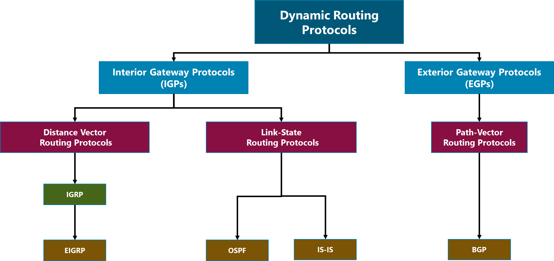
Figure 7 Routing Protocols Classification
2.4.2.1 Dynamic Routing Protocols
Interior Gateway Protocols (IGP)
An Autonomous System (AS) or routing domain is the unit of the router policy. It refers to a single network or a group of networks controlled by a common network administrator (e.g. the NaaS Operator EPC network). The IGP enables automatic routing for networks within the same AS, which is also referred to as intra-AS routing. IGPs include Enhanced Interior Gateway Routing Protocol (EIGRP), Open Shortest Path First (OSPF), and Intermediate System to Intermediate System (IS-IS); and can be classified in two main categories based on the information they provide to route: Distance Vector and Link-State routing protocols.
The choice of the routing protocol to be implemented is generally based on the network operator capabilities and network size. For the NaaS Operator environment, OSPF and IS-IS are the recommended protocols. Further discussion of the protocols, pros and cons can be found in the Transport & IP Architecture Module.
Exterior Gateway Protocols (EGP)
EGPs are used for routing between autonomous systems, which is also referred to as inter-AS routing. Interconnection between service providers and large companies is performed using an EGP.
The Border Gateway Protocol (BGP) is the de-facto EGP and is the official routing protocol used on the Internet. Even though BGP is an inter-AS protocol, it can still be used inside an AS as a pipe to exchange BGP updates among gateway routers belonging to the same AS, thats why BGP always requires an IGP to operate. BGP connections inside an AS are called Internal BGP (IBGP), whereas BGP connections between ASs are called External BGP (EBGP).
Figure 8 shows a BGP example where router R2 is receiving routing advertisements from R1, since the AS between R1 & R2 are different, R2 registers the routes into his routing table. When R3 receives the routing advertisements from R2, it discards the ones that belong to the same AS (AS-2) and only forwards the routes from AS-1 (acting as a pipe for routing advertisements).

Figure 8 EBGP and IBGP application diagram
BGP allows for easy traffic manipulation, so the NaaS operator will use it when connecting to networks in domains out of the control of its own administration, for example, to an Internet Service Provider (ISP) and to customer MNOs. These external networks cannot be trusted so the exchanged information should be carefully controlled with routing policies. However, if the NaaS operator only has one connection to an external domain (e.g. ISP), BGP is not needed and the use of static routes can be an option to provide connectivity (not recommended).
2.5 Network Element (NE) Capacity Planning Guidelines
Capacity Planning is a process that estimates the requirements of the network according to the expected services, subscribers and number of connections to external networks. The NaaS Operator must execute a Capacity Planning process in order to dimension the equipment and interfaces according to its needs. To facilitate capacity planning the following sections will be explored:
2.5.1 Capacity Dimensioning
Capacity forecasting is the network planning stage aimed to calculate the network needs to obtain an effective network, both in terms of cost and performance. The steps of the dimensioning stage are:
It should be noted that the total traffic generated consists of the user plane traffic and the signaling generated by every connection/session.
Step 1. The services offered by the network and the number of subscribers will directly drive the total traffic that the network needs to handle. To ease the capacity planning process, it is strongly recommended to separate Control Plane (CP), and User Plane (UP) traffic.
The User Plane (UP) is deeply correlated to the number of subscribers, the to-be-offered services, service penetration and the service profile.
The Control Plane (CP) is driven from user behavior in terms of mobility, service usage frequency and durations of active and idle behavior.
Specific methodology for calculation is provided in section 3.2.
Step 2. The capacity estimation for every network element is linked through a direct relation of the maximum number of users at busy hours (peak rates) and the role of each mobile core element. For logical entities with control plane functionality (e.g. MME), the number of signaling operation requests will be the main driver. In contrast, the ones with user plane functionality (SGW, PGW), the session establishment and data forwarding will have a major impact. The methodology to estimate the capacity demand for network elements is presented in section 3.2.
Step 3. To calculate the number of required network elements (NE), it is necessary to run a quick survey of commercially available equipment to know an average capacity for each metric. Once the average metrics are known, the required network element quantity is calculated as shown in the following equation:

(Eq. 1)
Where ![]() is the NE quantity,
is the NE quantity, ![]() is the n-th metric for one NE estimated in Step 3,
is the n-th metric for one NE estimated in Step 3, ![]() is the n-th average metric for one NE and
is the n-th average metric for one NE and ![]() is the number of metrics one NE has (see Table 2).
is the number of metrics one NE has (see Table 2).
The most common dimensioning parameters for the EPC and PCC elements are shown in Table 2. It is important to mention that for some vendors the metrics can be simplified to number of active users and total subscribers. The next table contains the metrics for each EPC logical element:
|
Metric |
Units |
|
|
MME |
Simultaneously Attached Users (SAU) |
Subscribers |
|
Idle to active transition/second |
Transactions per second (Tps) |
|
|
Tracking Area Update Requests |
Tps |
|
|
Handover requests |
Tps |
|
|
SGW/PGW-C |
Number of Active Bearers/Sessions |
Bearers/Sessions |
|
Number of transactions completed in one second |
Tps |
|
|
SGW/PGW-U |
Data Forwarding Capacity |
Gbps |
|
HSS |
Number of Users Supported |
Subscribers |
|
PCRF |
Operation Capacity |
Tps |
|
OCS |
Number of subscribers to be record |
Subscribers |
|
Number of transactions completed in one second |
Tps |
|
|
OFCS |
Number of subscribers to be record |
Subscribers |
|
Number of transactions completed in one second |
Tps |
Table 2. EPC/PCC Dimensioning parameters
3 Functions & Methodologies (How-To)
This section discusses the methodologies to perform critical tasks/subtasks involved in the Mobile Core design process, such as Interconnection Requirements, Capacity Forecast, and VNF Dimensioning. These critical tasks will help in the E2E process to reach a successful HLD recommendation.
3.1 Interconnection Requirements Definition
The Tx & IP Architecture Module establishes the protocols to be used in each of the network domains (last-mile and aggregation). Additionally, this module examines the alternatives to implement connections within the core elements and connections to external networks.
Most of the requirements and, consequently, the networking protocols are given by the network that is required to interconnect. The Mobile Core Architecture Module defines the connections to other networks (e.g. Internet) and through roaming agreements (to other MNOs). In this section, networking protocols for those interconnections are defined.
It is strongly recommended that the NaaS Operator implements the most common L2 & L3 protocols since this will facilitate interconnection. However, when interconnecting to legacy 2G/3G networks, some legacy protocols may be required.
The networking protocols can be subdivided into the following groups:
3.1.1 Layer 2 Recommendation
For Layer 2 (L2), even though there are several options to choose, the most conventional protocol is Ethernet and it can be over copper or fiber optic. It is always recommended to use Ethernet, thus avoiding interoperability issues.
In terms of VLAN segmentation, it is recommended to allocate VLANs for specific purposes such as O&M, or EPC interfaces. The recommendation should look as follows:
It is also recommended that the VLAN assignment for the MME follow the guidelines of the Tx HLD Module.
3.1.2 Layer 3 Recommendation
In terms of Layer 3 (L3), the most standardized protocol is Internet Protocol (IP). Routing protocols Open Shortest Path First (OSPF), Border Gateway Protocol (BGP) and Intermediate System to Intermediate System (IS-IS) operate at this layer together with IP. As stated in section 2.4.2, OSPF is recommended for Mobile Core internal routing in the NaaS environment due to its adaptability, flexibility and easiness of management. In addition, BGP should be considered by NaaS operators for boundary routing such as connection to other MNOs and to the Internet.
For example, for the EPC, the SGi interface is a 3GPP standardized point of connection between the Packet Data Network Gateway (PGW) and external networks (e.g Internet or IP Multimedia Subsystem, IMS). The SGi logical interface is based on Ethernet + IP protocols + BGP routing mechanism. In contrast, the connection between (Serving Gateway) SGW and PGW is the 3GPP-standardized interface S5/S8. The S5/S8 logical interface is based on Ethernet + IP protocols + IGP routing mechanism. Please refer to Figure 9.
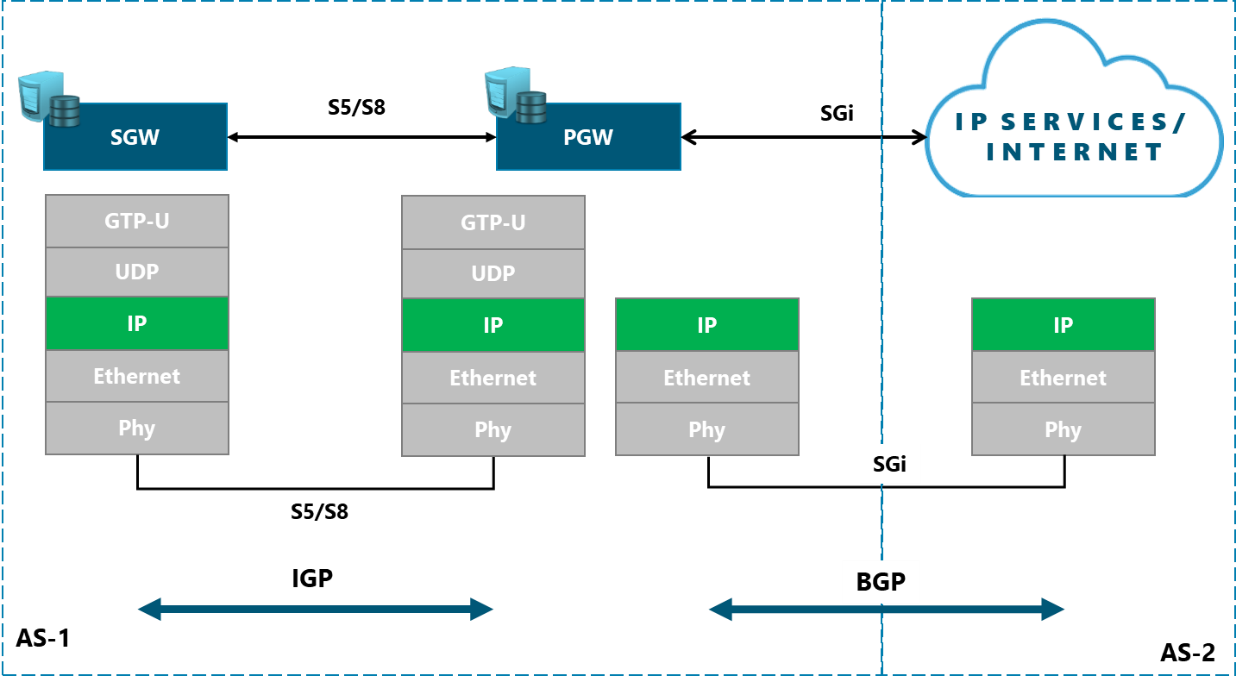
Figure 9 Layer 3 Recommendation for inner and outer EPC interfaces.
Security and privacy have always been a concern for all the networks and the EPC is not the exception. For connections within the EPC, it can be guaranteed that a certain degree of security and privacy is met because the infrastructure will be owned by the NaaS Operator. On the other hand, the connections to external networks will go through domains out of the control of the NaaS Operator so it is necessary to implement mechanisms to provide security to these outer connections.
Layer 3 Virtual Private Network (L3VPN) and IP Security (IPSec) are mechanisms to provide authentication and encryption of data packets between two network elements over the IP protocol. The advantages and disadvantages of L3VPN and IPSec are contained in the following table.
|
|
Pros |
Cons |
|
IPSec |
● Transparent to applications. ● No impact on higher layers. ● Can Apply to real-time traffic. ● IPSec offers encryption to: payload, header and routing information. |
● Since IPSec establishes a tunnel between two networks, the security breaches at IP level on the remote network are shared to the local network and vice versa. ● ISPs might consider anything IPSec-encrypted to be a "business-class" transmission and rate it at higher costs. ● Increased bandwidth and latency due to authentication and encryption process plus the IPSec overhead addition. ● NAT and Firewall might cause problems when IPSec is used. |
|
L3VPN |
● Extremely scalable VPN architecture. ● Allows the NaaS Operator to simplify its WAN routing by allowing direct routing information sharing between the equipment (router) on the edge of its own AS to the edge equipment of external networks or AS. ● Supports QoS and real-time traffic. ● Support tight SLAs with fast failover and guaranteed bandwidth. |
● Only IP traffic is supported which will result in lack of legacy protocol/ application support. ● Customers do not have complete control of their WAN IP routing. ● Customers must share the routing responsibility with the service provider. ● Do not natively (by default) offer the strong authentication and encryption of secure VPNs such as IPsec. |
Table 3. IPSec and L3VPN Pros and Con
In terms of security IPSec or L3VPN are largely supported and recommended, especially when connecting to external networks.
Further details of L3 routing mechanisms can be found in section 2.4.2.
3.1.3 Layer 4 Recommendation
There are only a few Layer 4 (L4) protocols commonly used. Transmission Control Protocol (TCP), User Datagram Protocol (UDP) and Stream Control Transmission Protocol (SCTP)
User traffic usually makes use of TCP or UDP and this should be transparent to the Mobile Core Network.
On the other hand, protocols to be used for signaling traffic may be defined by 3GPP standards and the NaaS Operator cant change them. Here, its important to note that some signaling interfaces by standard, require the use of Stream Control Transmission Protocol (SCTP). Whenever the NaaS Operator can choose the L4 protocol in a signaling interface, SCTP should be selected over TCP, because it has the same functionality plus enhanced capabilities.
3.1.4 Upper Layers Recommendation
GPRS Tunnel Protocol (GTP) and Diameter protocols are specified by 3GPP standards to be used in several Mobile Core interfaces on top of Layer 4. GTP is used for general communication and signaling (Control/User Plane), whereas Diameter is mainly used for authentication, authorization and accounting (AAA).
One of the most important scenarios where these protocols are required is for roaming. In home routed scenarios S6a (Diameter-based) and S8 (GTP-based) interfaces are required while in local breakout S6a and S9 (Diameter-based) are needed.
Diameter-based Interfaces
Diameter Edge Agent (DEA)/ Diameter Routing Agent (DRA) is an entity with routing capabilities at the Diameter layer. DEA/DRAs are required for diameter-based equipment for successful roaming interconnection since it will forward the diameter messages to the correct equipment. In other words, it means that for all external connections that are based on the diameter protocol, it is recommended to implement a single DRA.
Figure 10 shows the typical protocol stack for diameter-based interfaces such as S9 (Home to Visitor PCRF), S6a (MME to HSS) and Gx (PGW to PCRF) with an intermediate DRA.
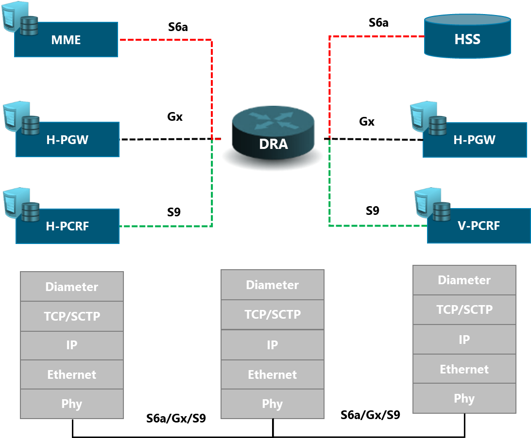
Figure 10 Typical Networking with a DRA.
For GTP, no requirements are needed since GTP is ready to cope with external and internal networks. For further configuration details, please refer to Mobile Core LLD Module.
Figure 11 and Figure 12 shows the typical protocol stacks for external and roaming interfaces where GTP is used.
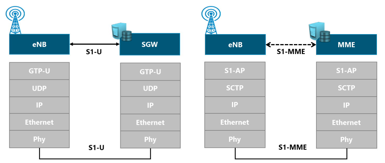
Figure 11 Protocol Stacks for an eNB connection to the EPC (MME and SGW).
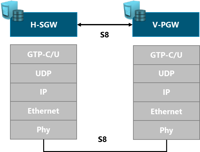
Figure 12 Protocol Stacks for external networks.
3.2 Capacity Forecast Analysis
Capacity forecasting is a process that uses subscriber forecasts from the RAN & Tx HLD Modules to estimate EPC Core interface and equipment dimensioning.
The inputs to perform capacity forecast are shown in Table 4. These inputs can be obtained from the RAN & TX HLD Modules and, in most cases, from other networks or estimates shared by the customer MNOs. If these are not available, values in the example presented throughout section 4.2 can be used.
|
Description |
|
|
|
Total number of users in the network, including those from customer MNOs [users] |
|
|
Percentage of the overall users that are users of a specific service [%] |
|
|
Percentage of active users during the busy hour [%] (can be applied to specific scenarios, e.g. active subscribers due to voice or data service). |
|
|
Percentage of Simultaneous Attached Users (SAU) during the busy hour [%] (SAU have at least one active/idle session established) |
|
|
Average data transmitted in a session at busy hour for a given service [MB/session] |
|
|
Number of sessions per user at busy hour [sessions] |
|
|
Average number of attach attempts per user at busy hour [transaction/user] |
|
|
Average number of detach attempts per user at busy hour [transaction/user] |
|
|
Average number of bearer activation/deactivation operations per user at the busy hour [transaction/user] |
|
|
Average number of idle/active transitions per user at the busy hour[transaction/user] |
|
|
Average number of Tracking Area Updates (TAU) procedures per user at busy hour [transaction/user] |
|
|
Average number of HO procedures attempted per user at busy hour [transaction/user] |
Table 4. Inputs for Capacity Forecast Analysis
Often, Mobile Core Solution Providers only require the total Number of Users ![]() and Number of active users during the busy hour
and Number of active users during the busy hour ![]() to dimension the solution. However, for more detailed dimensioning, the NaaS operator can follow the process described in the subsequent sections, which addresses the dimensioning of traffic, signaling, Mobile Core NEs and interfaces. As a complement, the Mobile Core Capacity Forecast Widget is provided to NaaS Operators to facilitate all the calculations related to Capacity Forecasting.
to dimension the solution. However, for more detailed dimensioning, the NaaS operator can follow the process described in the subsequent sections, which addresses the dimensioning of traffic, signaling, Mobile Core NEs and interfaces. As a complement, the Mobile Core Capacity Forecast Widget is provided to NaaS Operators to facilitate all the calculations related to Capacity Forecasting.
3.2.1 Traffic Dimensioning
Traffic Dimensioning estimates the total traffic generated by the total expected users. It is the input to calculate the forwarding capacity of the SGW and PGW entities and, additionally, S1-U, SGi and S5/S8 Interfaces.
Step 1. Users per service.
Capacity planning must begin with the user forecast from RAN HLD Module and penetration for each service such as data and voice. For a given service, the relationship to the estimated users is given by the following formula:
![]()
(Eq. 2)
Where: ![]() is the number of users for a given service in the network [users].
is the number of users for a given service in the network [users].
Step 2. Service Profile.
Each service will have a specific traffic model, it will depend on the frequency of usage (![]() ) and the amount of data transferred in every session (
) and the amount of data transferred in every session (![]() ). The next equation shows this relationship:
). The next equation shows this relationship:
![]()
(Eq. 3)
Where: ![]() is the amount of data per service per user at busy hour [MB].
is the amount of data per service per user at busy hour [MB].
After calculating the total amount for each service, it is necessary to translate into bandwidth by the next equation:
![]()
(Eq. 4)
Where: ![]() is the bandwidth per user for a specific offered service at busy hour [Mbps].
is the bandwidth per user for a specific offered service at busy hour [Mbps].
Step 2. Data Traffic.
The total data traffic (![]() ) is calculated by the sum of the products of the service bandwidth (
) is calculated by the sum of the products of the service bandwidth (![]() ) and the active users per service (
) and the active users per service (![]() ) at the busy hour. This calculation will help the NaaS Operator to estimate the traffic that will go through interfaces such as S1-U, S5/S8 and SGi.
) at the busy hour. This calculation will help the NaaS Operator to estimate the traffic that will go through interfaces such as S1-U, S5/S8 and SGi.
First, the active users per service at busy hour are calculated as follows:
![]()
(Eq. 5)
Then the total data traffic (![]() ):
):
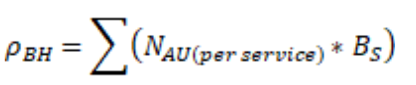
(Eq. 6)
Where ![]() is measured in Mbps.
is measured in Mbps.
3.2.2 Signaling Dimensioning
The Signaling dimensioning estimates the total amount of signaling load generated by the users due to registration, mobility, security and session establishment procedures. The first step is to calculate the number of simultaneous attached users (![]() )
)
![]()
(Eq. 7)
Then, the signaling calculation (number of transactions per second) must be based on this number of simultaneous attached users multiplied by the number of attempts for a given signaling procedure at peak hours. For Attach procedures:
![]()
(Eq. 8)
Where: ![]() is the average number of attach attempts per user at busy hour [transaction/user] and
is the average number of attach attempts per user at busy hour [transaction/user] and ![]() is the total number of attach procedures [transaction/hr].
is the total number of attach procedures [transaction/hr].
For Detach procedures:
![]()
(Eq. 9)
Where: ![]() is the average number of detach attempts per user at busy hour [transaction/user] and
is the average number of detach attempts per user at busy hour [transaction/user] and ![]() is the total number of detach procedures [transaction/hr].
is the total number of detach procedures [transaction/hr].
For Bearer establishment and termination procedures:
![]()
(Eq. 10)
Where: ![]() is the average number of Bearer establishment attempts per user at busy hour [transaction/user] and
is the average number of Bearer establishment attempts per user at busy hour [transaction/user] and ![]() is the total number of Bearer establishment procedures [transaction/hr].
is the total number of Bearer establishment procedures [transaction/hr].
For Bearer Modification and termination procedures:
![]()
(Eq. 11)
Where: ![]() is the average number of Bearer modification attempts per user at busy hour [transaction/user] and
is the average number of Bearer modification attempts per user at busy hour [transaction/user] and ![]() is the total number of Bearer modification procedures [transaction/hr].
is the total number of Bearer modification procedures [transaction/hr].
For Tracking Area Update procedures:
![]()
(Eq. 12)
Where: ![]() is the average number of TAU attempts per user at busy hour [transaction/user] and
is the average number of TAU attempts per user at busy hour [transaction/user] and ![]() is the total number of TAU procedures [transaction/hr].
is the total number of TAU procedures [transaction/hr].
For Handover procedures:
![]()
(Eq. 13)
Where: ![]() is the average number of handover attempts per user at busy hour [transaction/user] and
is the average number of handover attempts per user at busy hour [transaction/user] and ![]() is the total number of handover procedures [transaction/hr].
is the total number of handover procedures [transaction/hr].
For Idle to Active state transition procedures:
![]()
(Eq. 14)
Where: ![]() is the average number of active/idle state transition attempts per user at busy hour [transaction/user] and
is the average number of active/idle state transition attempts per user at busy hour [transaction/user] and ![]() is the total number of active/idle state transition procedures [transaction/hr].
is the total number of active/idle state transition procedures [transaction/hr].
In the end, the sum of all the procedures that occur at the busy hour per logical entity will drive the dimensioning and these procedures must not surpass the 80% capacity of each logical entity. For example, for the MME, the following equation applies:
![]()
(Eq. 15)
Where ![]() is the total number of procedures at busy hour at a specific interface or logical entity [transaction/hr]. Guidance to modify the equation above for other logical entities is provided in the example in section 4.2
is the total number of procedures at busy hour at a specific interface or logical entity [transaction/hr]. Guidance to modify the equation above for other logical entities is provided in the example in section 4.2
Finally, the only method to know the number of occurrences is to measure in live network these average numbers, but considering the EPC is a new deployment, a good estimation of occurrences per user at busy hour is contained in Table 5. It is based on user behavior from other networks.
|
Average number of Occurrence per user per hour |
|
|
Attach ( |
1 |
|
Detach ( |
1 |
|
Idle to active transition ( |
5 |
|
Bearer Establishment ( |
0.5 |
|
Bearer Modification ( |
0.1 |
|
Tracking Area Update ( |
0.3 |
|
Handover ( |
0.2 |
Table 5 Occurrences for every type of signaling procedure
3.2.3 Interface Dimensioning
Interface Dimensioning calculates the total amount of traffic of each EPC logical interface according to the corresponding signaling procedures and data forwarding (CP+UP).
Control Plane (CP):
The CP is where all the signaling procedures are carried out so for the traffic load calculation it is assumed that for every procedure attempt 100 KB are used. Under this premise, we can calculate the bandwidth that the signaling is generating in every external interface. The interfaces are characterized by the type of signaling procedures they support:
For S1-MME Interface:
For S6a Interface:
For S8 Interface:
For S9 Interface:
The equation for calculating the amount of signaling traffic is the same for all the above interfaces.

(Eq. 16)
Where: ![]() is the Interface Control Plane [kbps],
is the Interface Control Plane [kbps], ![]() are the Signaling Messages per subscriber at busy hour at a given interface [messages/subscriber/hour].
are the Signaling Messages per subscriber at busy hour at a given interface [messages/subscriber/hour].
For example, for S1-MME interface assuming a ![]() of 50% for 10k users.
of 50% for 10k users.
![]()
S1-MME will have Attach, Detach, Idle to active state change, TAU & Handover procedures so based on Table 5.
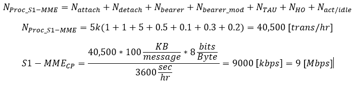
User Plane (UP):
The only interfaces who carry UP traffic are: S1-U, S5/S8 and SGi. These interfaces will carry the data from all the users towards the Internet so the user traffic load will be the same in non-roaming scenarios.
![]()
(Eq. 17)
For roaming scenarios, there are two possible options:
1 Local Breakout:
The interfaces that will be connected to other MNOs networks are S6a and S9 as shown in Figure 13. This will have no impact on the previous equation.
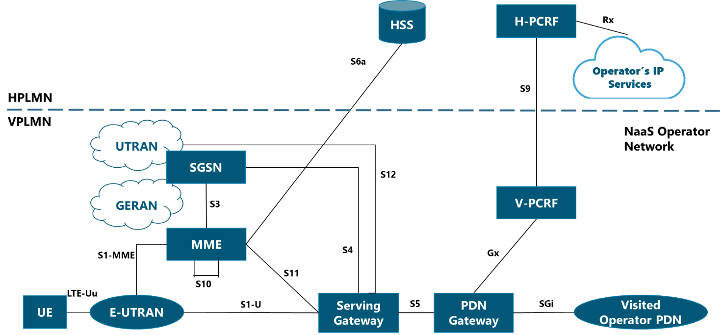
Figure 13 Local breakout architecture.
2 Home Routed:
The interfaces that will be connected to other MNOs networks are S6a and S8 as shown in Figure 14.
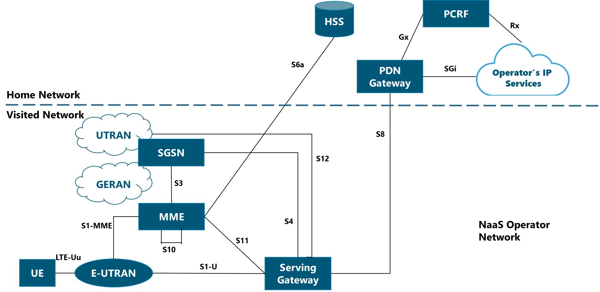
Figure 14 Home Routed Roaming Architecture.
For this scenario, the S8 interface will carry the user traffic and signaling to other MNO networks and it should be calculated based on the roaming subscribers:
![]()
(Eq. 18)
Where: ![]() is the number of active users which correspond to roaming.
is the number of active users which correspond to roaming.
The load of the S5 and SGi interfaces on the NaaS Operator EPC will decrease due the S8 traffic redirection to the corresponding MNOs. The equation (16) will transform into:
![]()
(Eq. 19)
Where: ![]() is the total traffic throughput corresponding to the S5 and SGi interfaces in the home-routed roaming scenario.
is the total traffic throughput corresponding to the S5 and SGi interfaces in the home-routed roaming scenario.
3.3 VNF Dimensioning
After Capacity Dimensioning is done, the following step is mapping these requirements to VNFs. There are three steps for VNF Dimensioning. First, the minimum VNF requirements according to each type of VNF need to be defined. Second, the selection of the VNF Mapping option (if possible) according to vendors offering and NaaS Operator requirements. Third, the VNF/NE mapping where it is defined the number of VNFs or NEs.
3.3.1 VNF Requirements definition
The EPC elements are needed to be mapped to VNFs, but the type of VNFs (CP, UP or Database) is assigned according to the type of NE is serving. For example, UP VNFs can be mapped to logical entities such as SGW or PGW. The VNFs for the EPC are divided into the following categories:
Where:
3.3.2 VNF Mapping
Once the traffic estimation for all planes in the logical equipment is done, the mapping into Virtual Network Functions (VNF) can be performed. There are several approaches when doing it:
|
Mapping Type [VNF:NE] |
Description |
Advantages |
Disadvantages |
|
1:1 |
Each VNF will contain 1 NE. |
Easy Capacity match Mid level of reliability |
Less Flexible |
|
1:N |
1 VNF will handle several NE. The capacity of the VNF must meet all the NE requirements. |
Less Number of VNFs |
Reduced Flexibility & Adaptiveness Limited Scaling capacity Low level of reliability due to single point of failure |
|
N:1 |
1 NE will be divided into N VNF. The division can be in terms of networking, processing or data forwarding capacities. |
Improved Flexibility & Performance Resource Efficient VNF per service Granularity High level of reliability |
Greater number of VNFs to handle |
Table 6. VNF to NE Mapping Available Options
Most of the time, this mapping is not offered by the vendors as a selection since they may have already defined one beforehand. For the options which the NaaS Operator can select a type of mapping, it is recommended to choose one in the following order: N:1, 1:1 and 1:N.
3.3.3 VNF/Network Element Dimensioning
After the calculation of the user traffic amount and signaling, it is mandatory to map the corresponding metrics into logical entities such as MME, HSS, SGW, PGW (or VNFs representing them). If the solution is a core-in-a-box type, the calculation must be based on the metrics the solution provides, but the logic is the same for quantity calculation.
For logical entity quantification, it is necessary to know the specification from vendors of the maximum load that an entity can bear in terms of simultaneous attached users (![]() ) and signaling handling load (
) and signaling handling load (![]() ). Below, formulas used to estimate the amount of logical entities are presented.
). Below, formulas used to estimate the amount of logical entities are presented.
The signaling procedures that the logical entities must cope with are given by the following relationships:
For HSS ![]() , it must be considered:
, it must be considered:
For MME ![]() , it must be considered:
, it must be considered:
For SPGW ![]() , it must be considered:
, it must be considered:
HSS dimensioning:
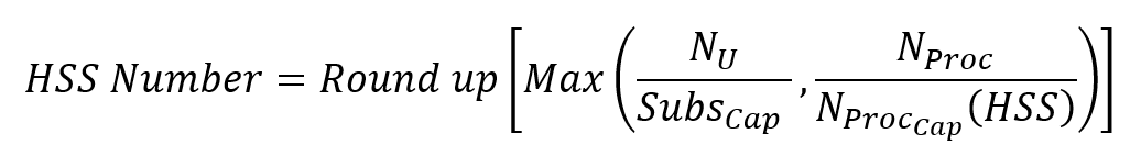
(Eq. 20)
Where: ![]() is the Subscriber Capacity of the HSS [users/HSS] and
is the Subscriber Capacity of the HSS [users/HSS] and ![]() is the maximum capacity for signaling handling of the HSS [trans/sec/HSS].
is the maximum capacity for signaling handling of the HSS [trans/sec/HSS].
MME Dimensioning:

(Eq. 21)
Where: ![]() is the Simultaneous Attached Users Capacity of the MME [users/MME] and
is the Simultaneous Attached Users Capacity of the MME [users/MME] and ![]() is the maximum capacity for signaling handling of the MME [trans/sec/MME].
is the maximum capacity for signaling handling of the MME [trans/sec/MME].
SGW/PGW Dimensioning:

(Eq. 22)
Where: ![]() is the Maximum Bearer handling capacity of the S/PGW [bearer/SGW or PGW] and
is the Maximum Bearer handling capacity of the S/PGW [bearer/SGW or PGW] and ![]() is the maximum capacity for signaling handling of the S/PGW [trans/sec/ SGW or PGW].
is the maximum capacity for signaling handling of the S/PGW [trans/sec/ SGW or PGW].
4 E2E Process Flow
This section presents an end-to-end process to perform a High-Level Design for the Mobile Core Network. This process is generic and it will suit most of the requirements of the NaaS Operator, further customization can be added to deliver a better design to each NaaS Operator scenario. The steps of the E2E flow will be discussed in the upcoming sections.
4.1 End-to-end Process Overview
As presented in Figure 15, the end-to-end process consists of four main steps.
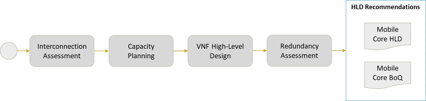
Figure 15 Module Functional View
The first step is the Interconnection Assessment, in which the NaaS Operator selects the best networking protocols and entities when connecting to external networks. As this step defines the general network description and function, it is the strongest input-dependent and its output provides significant insights to the next processes.
Capacity Planning consists of the calculation of the forecasted traffic on the interfaces and logical elements of the mobile core network based on the RAN HLD forecasted users and traffic information combined with the mobile core architecture input.
VNF High Level Design comprises the estimation of the VNF dimensioning and the Bill of Quantities (BoQ) corresponding to the mapping into logical entities.
Finally, the redundancy assessment primarily involves the evaluation and guide to select the redundancy and availability mechanisms.
4.2 Step-by-step Analysis
In this section, each of the steps in the E2E process are examined to provide practical guidance for NaaS Operators, describing the range of implementation options. The steps can be further customized according to the NaaS Operator requirements and constraints.
In order to facilitate understanding of the process design flow, a Design Example is followed along each of the process steps. Before getting into the details of the process, an overview of the design example scenario is presented.
Design Example: Scenario Definition
In this example, the process to generate the HLD Design for a NaaS Operator which will initially own 500k subscribers and will provide service to one MNO through a home-routed roaming scheme. EPC architecture is shown in Figure 16.

Figure 16. Design Example Scenario.
Inputs for this scenario are detailed below:
-Elements to be deployed: MME, SGW, PCRF, PGW, HSS and DRA (yellow equipment).
-Home-routed Roaming scenario
-Voice service: VoIP-only.
-Subscriber Forecast (NaaS) (![]() ): 500,000 users + 100,000 forecasted over the next two years.
): 500,000 users + 100,000 forecasted over the next two years.
-Subscriber Forecast (MNO #1) (![]() for roaming): 50,000 users.
for roaming): 50,000 users.
-Percentage of Simultaneous Attached Users (![]() ): 50 %.
): 50 %.
Service Details:
-Data Service Penetration (![]() for Data): 100 % of the users
for Data): 100 % of the users
-Voice Service Penetration (![]() for Voice): 100 % of the users
for Voice): 100 % of the users
–User behavior (![]() ):
):
50% Data Usage at peak hours.
20% Voice Usage at peak hours
Based on other networks traffic models, the following traffic model is assumed for Voice and Data Services:

After a quick survey from vendors:
– NE Capacity Characteristics:
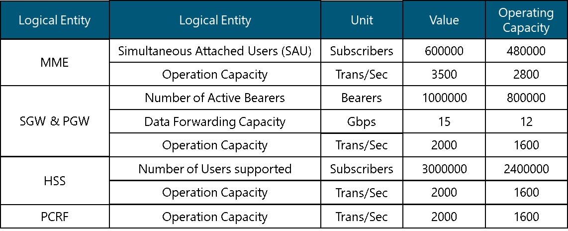
4.2.1 Interconnection Assessment
The steps will help to select the best networking protocols and entities when connecting to external networks towards a successful interconnection.
Step 1. Select the most appropriate Networking protocols.
For L2, the most commonly used protocol is Ethernet.
For L3, we have a variety of internal routing protocols such as IS-IS, OSPF. The operator should select one from section 2.4.2 according to the needs and the capabilities of the NaaS Operator. In the case of exterior routing protocols, we only have BGP which will be used when connecting to external networks such as the Internet.
For L4, the selection between TCP, UDP and SCTP is simple since most of the standardized interfaces already define the L4 protocol to be used, see section 3.1.3.
Step 2. Selection of Upper Layer protocols for interconnection.
As stated in section 3.1, there are two groups of interfaces depending on the protocol they use: GTP and Diameter. When connecting to external networks only diameter has an impact on the design.
For Diameter-based external interconnections the use of DRA is always recommended and must be implemented. For internal diameter connections, the use of DRA is optional.
Design Example
Step 1. Since there is no special requirement from the Mobile Core Architecture to support legacy protocols nor limitations on routing and switching, the selection of networking protocols is:
L2 Protocols: Ethernet
L3 Protocols: IP (OSPF + BGP)
L4 Protocols: Given by interface specification.
SCTP: S1-MME & S6a.
TCP/UDP: S1-U & S8.
Step 2. From the topology, it can be seen that it will need a S8 interface between the home SGW to Visitor PGW. Additionally, a diameter-based S6a from the home MME to the Visitor HSS.
For GTP:
S8 interface is GTP and it does not need any special requirement
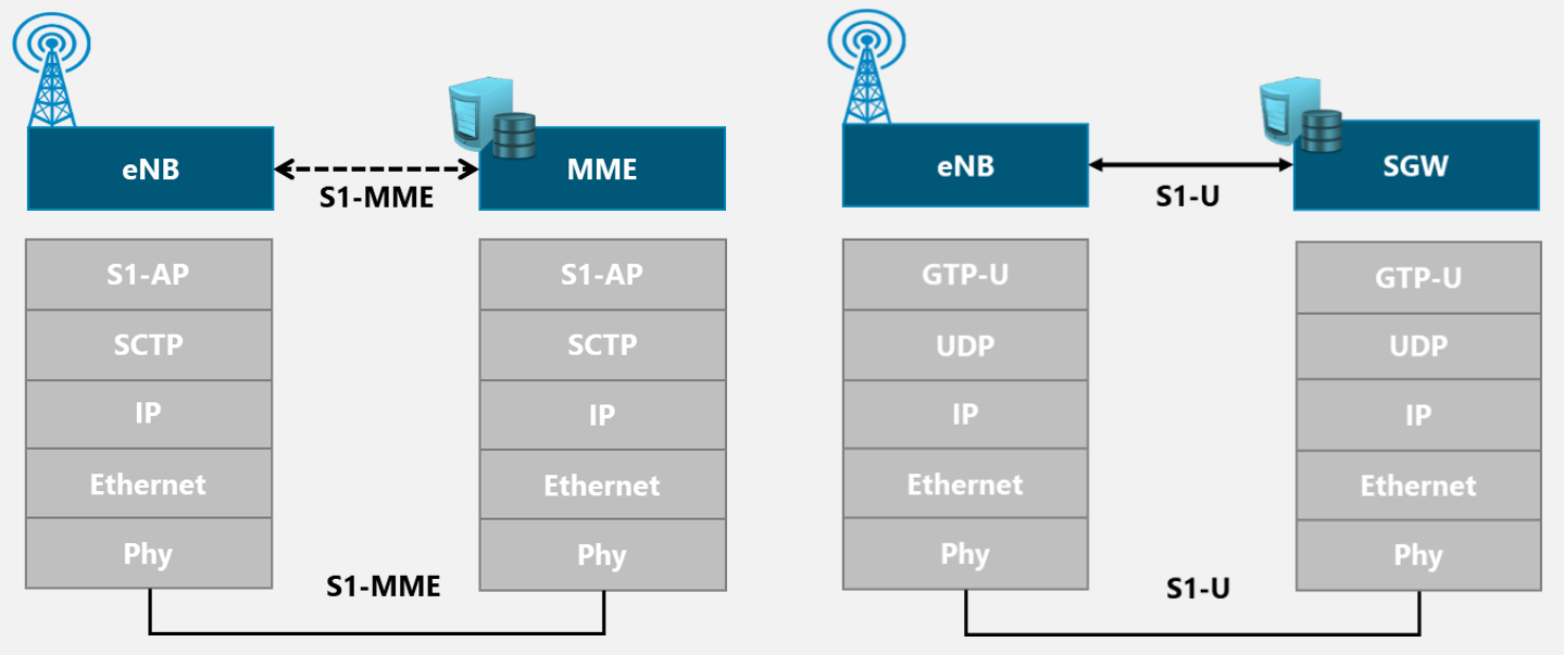
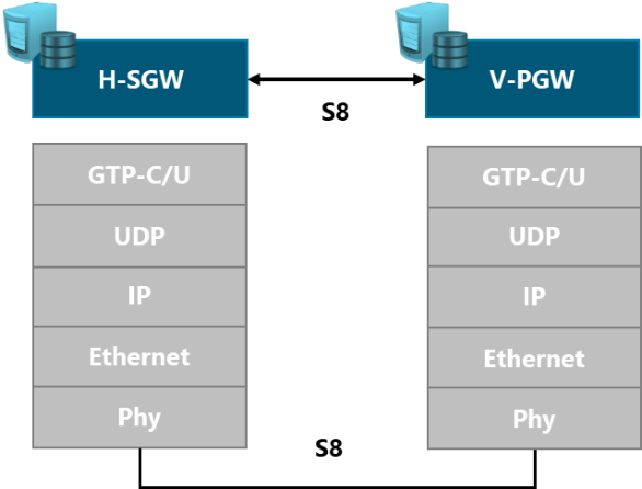
For Diameter:
Implementation of DRA for S6a signaling messages between MME and two HSS (local and visitor).
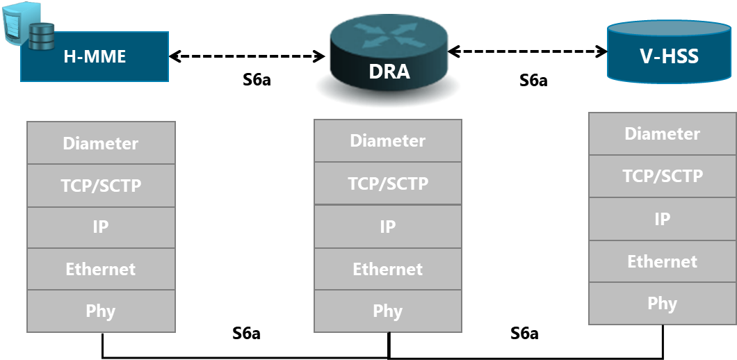
Finally, SGi:
Since the L3 protocol is already selected, no need to further selection on the SGi interface.
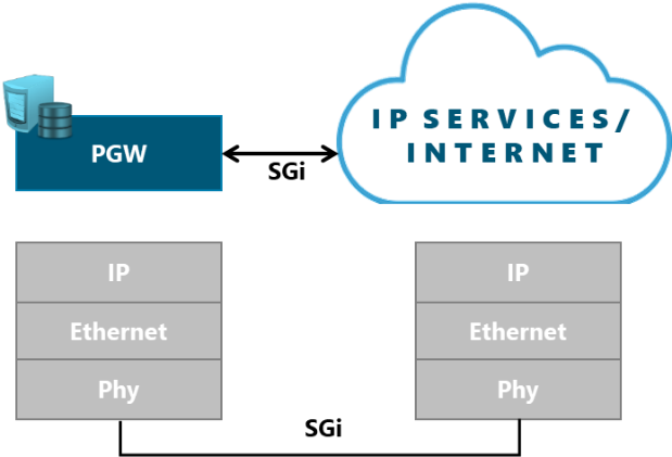
4.2.2 Capacity Planning
The objective of this step is to perform the capacity calculation for each element and interface based on the user traffic model.
Traffic Dimensioning estimates the total traffic generated by the total expected users. It will be used for interface and logical entities dimensioning. Through these steps, the following metrics are calculated following the methodology in section 3.2.1:
Step 2. Signaling Dimensioning
The Signaling dimensioning estimates the total amount of signaling load the users are generating due to registration, mobility, security and session establishment procedures. Based on the methodology presented in section 3.2.2, the following metrics are the output for this step:
Step 3. Interface Dimensioning
Interface Dimensioning calculates the total amount of traffic of each EPC logical interface according to the corresponding signaling procedures and data forwarding (CP+UP). It will be used for interface and logical entities dimensioning. The following metrics are the output for this step, which are calculated as described in section 3.2.3:
A useful widget for all the calculations related to Capacity Planning can be found on the Mobile Core Capacity Forecast Widget.
Design Example
Step 1. Traffic Dimensioning
The first step is to calculate the total number of users. The following formula considers the expected users, the forecasted users and the roaming expected users as well.
![]()
The next step is to calculate the number of users per service. The total users for Data Services:
![]()
The total users for Voice Services:
![]()
Number of active users at peak hours for data and voice, respectively:
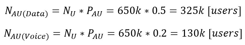
For Voice and Data Services, the following traffic model is used. It is based on the average user behavior on other live networks.
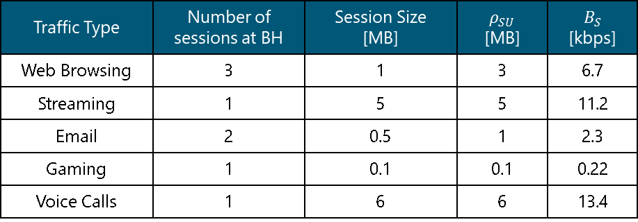
The traffic types of Web Browsing, Streaming, Email and Gaming correspond to Data services while Voice Calls corresponds to Voice services. So the bandwidths are:
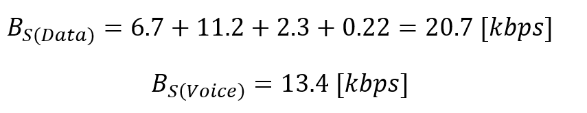
Total bandwidth usage for the internet connection:
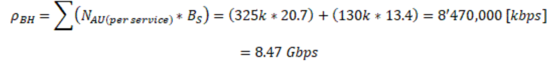
Step 2. Signaling Dimensioning
The first step is calculating the Simultaneous Attached Users for calculating the number of signaling procedures. To calculate the Simultaneous Attached Users:
![]()
From table 1 we can get the average number of occurrences for each connected subscriber. The calculation is it done to the following signaling procedures and then calculated on transactions per second:
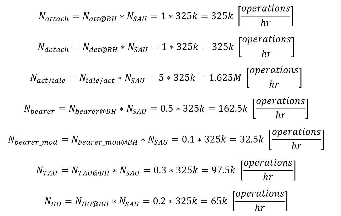
Step 3. Interface Dimensioning
For Control Plane interfaces (S1-MME and S5/S8) since we already calculated the operations per second in step 3:
For S1-MME:
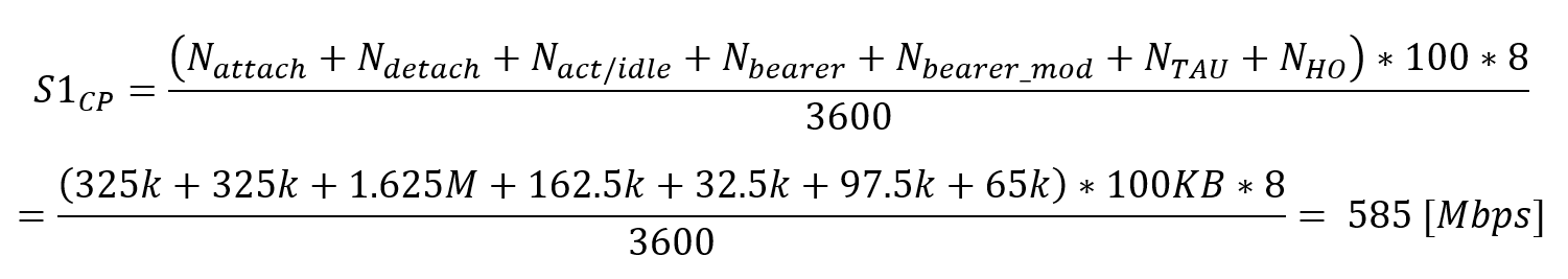
For S5/S8:
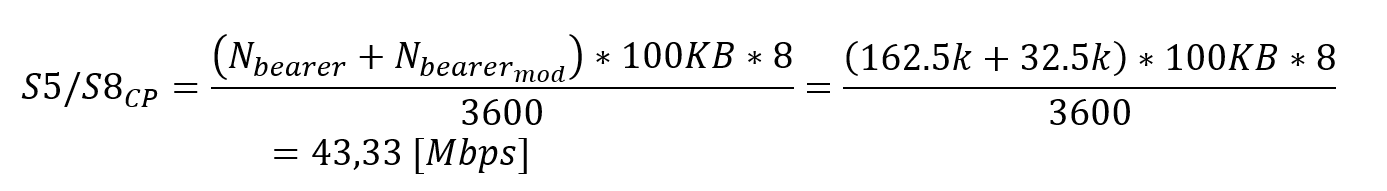
For User Plane interfaces (S1-U, S5/S8 and SGi):
For S1-U:
![]()
Since it is a Home Routed scheme for roaming:
For S8:
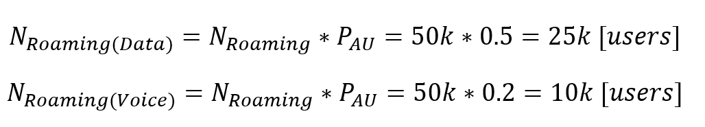
So the total traffic for the S8 user plane is:
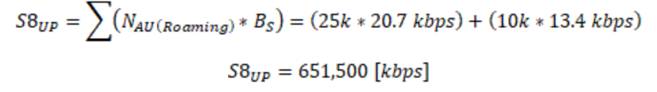
For S5 & SGi (Since it is home routed roaming scenario):
![]()
Summary:
Finally, for interfaces which have a UP and CP, the total loads must be summed up:
For S5:
![]()
For S8:
![]()
The following table summarizes for all the external interfaces and expresses the capacities in Mbps:
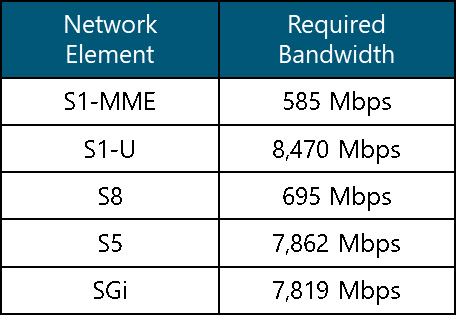
4.2.3 VNF High Level Design
For the VNF High Level Design, three aspects must be defined: VNF Requirements, Type of VNF Mapping and VNF/NE Dimensioning.
VNF Requirements: From section 3.3.1, the mandatory specifications for each VNF is contained. These mandatory characteristics should be matched when it is possible to select from the vendors options. In the case that core-in-a-box option or 1:1 Mapping option is going to be implemented, the collective mandatory requirements should be matched by the solution.
Type of VNF Mapping: As seen in section 3.3.2, the advantages and disadvantages should drive the decision. For the options which the NaaS Operator can select a type of mapping, it is recommended to choose one in the following order: N:1, 1:1 and 1:N.
If several options are available for one mapping selection, a VNF/NE dimension can be performed before this decision is made.
VNF/NE Dimensioning: The section 3.3.3 indicated how is the process to follow to calculate the number of VNF or NE (depending on the mapping option). If the mapping option is not already chosen, a VNF dimensioning can be performed to help deciding.
Design Example
VNF Requirements:
From section 3.2, it is recommended to match these mandatory requirements to the VNF from available vendors when selecting a virtualized solution.
The VNFs for the User Plane must have Hyperthreading support and SR-IOV/DPDK. The VNFs that include the User Plane type are the SGW and PGW VNFs.
The VNFs for the Control Plane must have Hyperthreading support. The VNFs that include the Control Plane type are the MME and PCRF VNFs.
Finally, the VNFs for Database must have High IOPS features. The VNFs that include the Database type are the HSS VNFs.
VNF Mapping:
As the vendor in this example does not allow to select the VNF Mapping and states in 1:1, this mapping option is selected.
VNF/NE Dimensioning: Logical Entities or VNFs Quantity Calculation. In this example, the only option is 1:1 so VNF and NE Quantity are the same.
For the logical entities modeling, the vendor provides the following metrics:

From section 3.3.3, the quantity calculation is based on the metric capacity at 80% (Operating Capacity) considering the total amount of user traffic and signaling loads:
For the HSS:
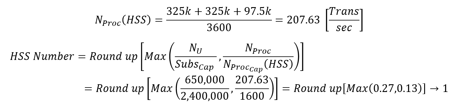
For the MME:
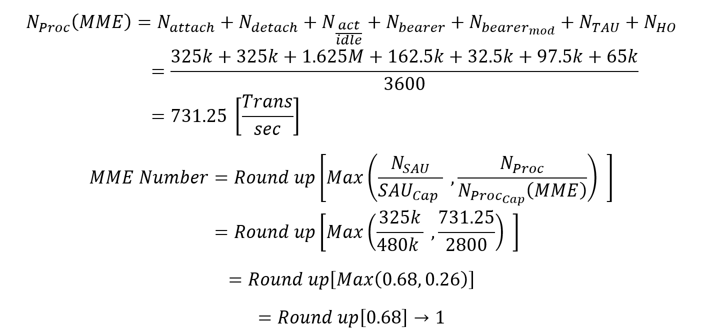
For the SGW & PGW:
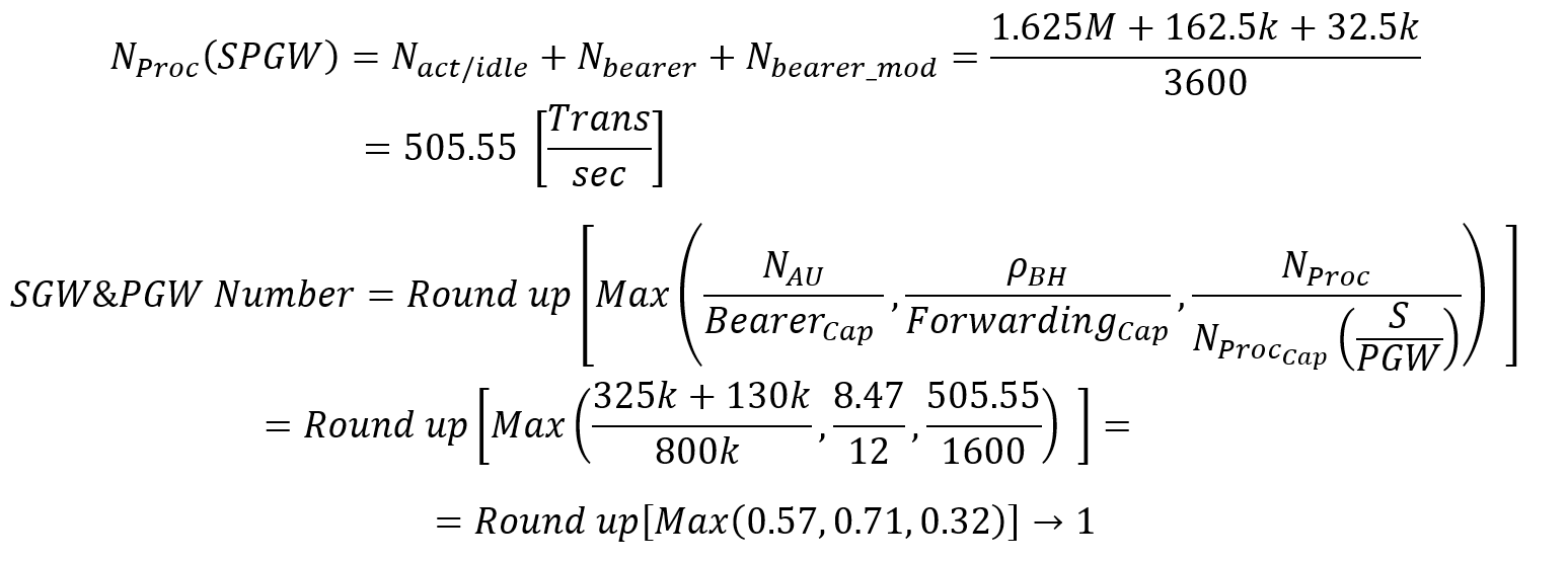
In the end, the numbers of required elements are:
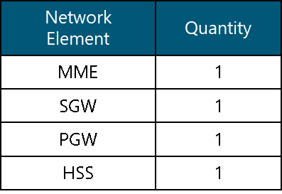
4.2.4 Redundancy Assessment
Redundancy on Mobile Core can be implemented on different levels and they can all be employed at the same time. Although this requirement comes from the Mobile Architecture Module, it can vary in the implementation approach. For all the available mechanisms, the major categories are:
- Hardware Level Resilience
- Application Level Resilience
Step 1. Selection of Hardware Level Resilience.
For the Mobile Core HLD, the only option that can be selected related to redundancy mechanisms is the networking characteristics. The reason is that at this point, no hardware has been selected and consequently, no storage scheme is defined.
For Network high availability: bonding mechanisms and physical redundancy schemes can be implemented (2N, N+M and N+1).
It is strongly recommended to implement a N+1 as a minimum for any non-crucial (S6a, Gx) interfaces and 2N scheme for the most important ones (e.g. S1-MME, S1-U, S5/S8, SGi).
Bonding mechanism is desired to act a group of physical interfaces as one.
Step 2. Selection of Application Level Resilience.
At the application layer, 2N, N+1 and N+M Redundancy are the options for VNF/NE redundancy and it can be applied in active/active and active/standby. For a small operator it might look excessive to deploy 2N or M+N models and prefer to develop a N+1. For further details, please refer to the Mobile Core Architecture Module.
It is recommended for the most important VNF to have 2N redundancy scheme (MME, SGW, PGW), whereas less crucial VNF can have N+1 application level redundancy.
Design Example
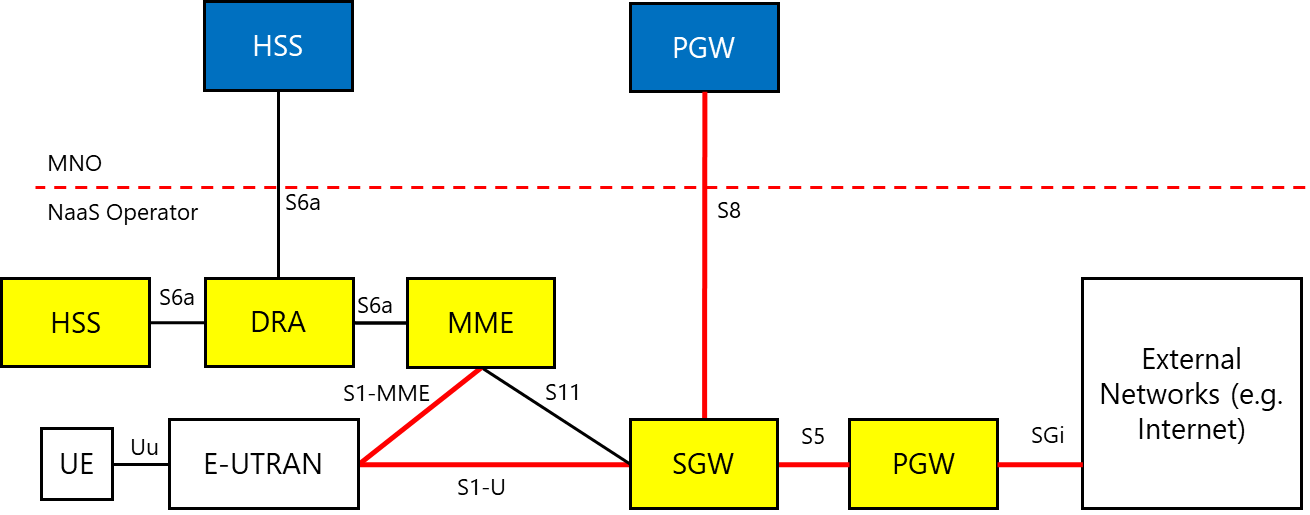
Step 1. Selection of Hardware Level Resilience.
For Network:
For each red interface (S1-MME, S1-U, S5, S8 and SGi), there will be a 2N redundancy since those are considered the most critical interfaces whereas the black ones (S11, S6a) can be implemented through N+1.
Based on 10 Gbps physical interfaces, it becomes clear that for S1-U (8,470 Mbps), S5 (7,862 Mbps) and SGi (7,819 Mpbs), a bonding mechanism is needed to make at least two physical interfaces to work in load sharing mode.
As a summary:
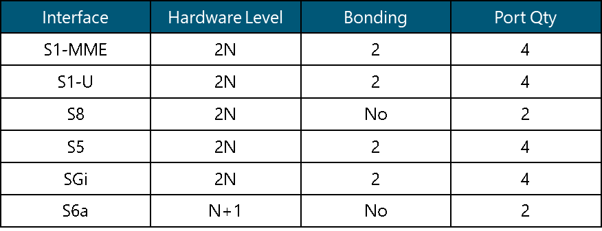
Step 2. Selection of Application Level Resilience
The MME, SGW and PGW will have 2N redundancy mechanisms. The HSS and DRA will have N+1 redundancy mechanism.
In summary:
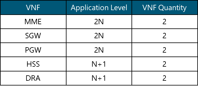
5 HLD Recommendation
This section presents a methodology to consolidate and generate a final HLD recommendation.
5.1 HLD Recommendation Format & Structure
The main deliverable of this module is the HLD recommendation which contains the overall technical solution, basic design rules, technologies and concepts required to describe Mobile Core Network. The HLD recommendation shall contain the following aspects:
5.2 HLD Recommendation Generation
The outputs of the end-to-end process will result in the generation HLD Recommendation. The BoQ can be generated according to the quantity outputs of the VNF High Level Design and the Redundancy Assessment processes.
The NaaS Operator can use the HLD Report Template as a reference for the format and structure of the final document. Further customization can be applied by the NaaS Operator in order to have a better and more personalized result.
1. Mobile Core LLD – Introduction
The Mobile Core Low-Level Design (LLD) module offers instruction on the key tasks for a detailed Mobile Core Design: IP Planning, Networking Parameter Design and the generation of the Core Network Bill of Materials (BOM). It also provides methodologies to design a virtualized implementation based on the HLD and the selected solution.
The LLD module provides recommendations on the parameter definition and configuration of all the Physical and Logical entities of the virtualized Evolved Packet Core (vEPC), specific protocols to enable enhanced functionalities supporting fault detection and improved routing capabilities, and resiliency and availability. An accurate Mobile Core LLD will lead to fewer fault occurrences due to missing configurations, greater probability to achieve the expected KPIs, and ease troubleshooting during the operations and maintenance phase.
The main output from using this module is the Mobile Core LLD Design which includes Equipment Selection and Dimensioning, Bill of Materials Generation, Physical & Logical Topology, IP Planning, and Routing & Switching Configuration. It also includes guidelines for configuration EPC Network Elements and Policy & Charging rules definition.
1.1 Module Objectives
This module will enable NaaS Operators to stand-up, run and manage a Mobile Core LLD initiative. The specific objectives of this module are to:
1.2 Module Framework
The Module Framework in Figure 1 describes the structure, interactions and dependencies among different NaaS operator areas.
Strategic Plan & Scope and High-Level Network Architecture drive the strategic decisions to forthcoming phases. Network Design is the first step into implementation strategy which is supported by Supply Chain Management.
The Mobile Core LLD module is included within the Network Design Stream and has a direct relation with Mobile Core HLD.
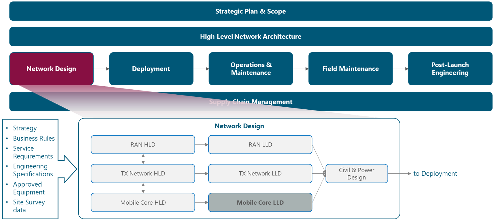
Figure 1. Module Framework
Figure 2 presents the Mobile Core LLD functional view, where the main functional components are exhibited. Critical module inputs are further described and examined. In addition, guidance and methodologies to execute the tasks included within each function are described in Section 3.
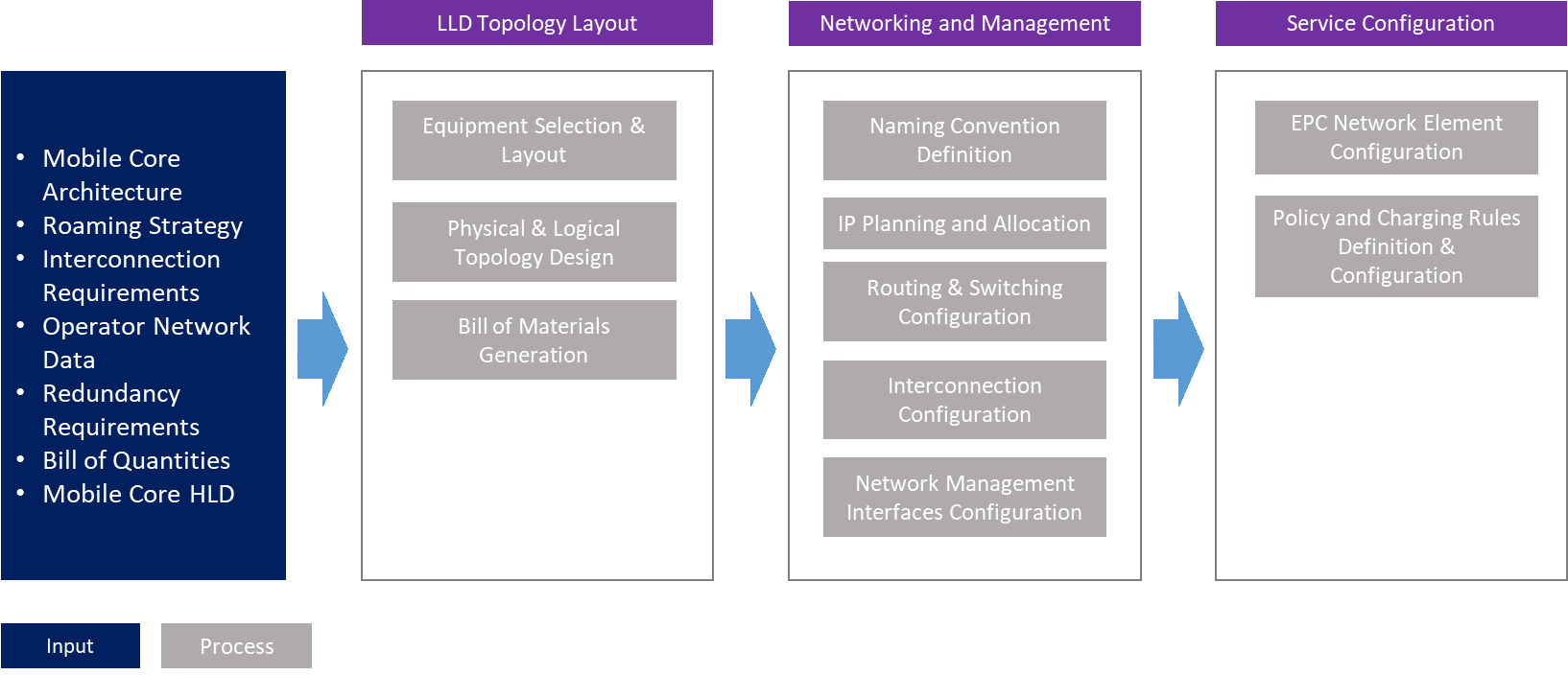
Figure 2. Module Functional View
The structure of the module is divided into four sections. Section 1 is a birds-eye view of the Mobile Core fundamentals involved in its design. Once fundamental knowledge is acquired, Section 2 focuses on showing a hands-on view of the tasks involved in the design. Section 3 organizes functional tasks on an end-to-end process flow that can be used as-is or be adapted by NaaS operators to match with their particular conditions. Finally, Section 4 illustrates how to integrate previous elements into a comprehensive Low-level Design (LLD) recommendation.
2 Mobile Core LLD Fundamentals
The Mobile Core Architecture Module defines the network architecture according to interconnection requirements from the NaaS Operator, its preexisting infrastructure and the services to be offered. Subsequently, in the Mobile Core HLD, the Dimensioning of the Equipment, Capacity Planning of the logical entities and a set of availability mechanisms and networking protocols were established in order to have a functional design of the EPC over a virtualized infrastructure.
Figure 3 depicts the typical EPC Architecture where it shows the Mobility Management Entity (MME), Serving and Packet Data Network (PDN) Gateways (SGW & PGW), the Home Subscriber Server (HSS) and the Policy and Charging Rules Function (PCRF) with the interconnection to the Evolved Universal Radio Access Network (E-UTRAN) and IP Networks (e.g. Internet, Enterprise Networks, etc.).
Connections to external networks may increase depending on the roaming agreements & defined approach, voice solution requirements, existing Packet Switched (PS) infrastructure and Multiple Network Operator (MNO) strategy.
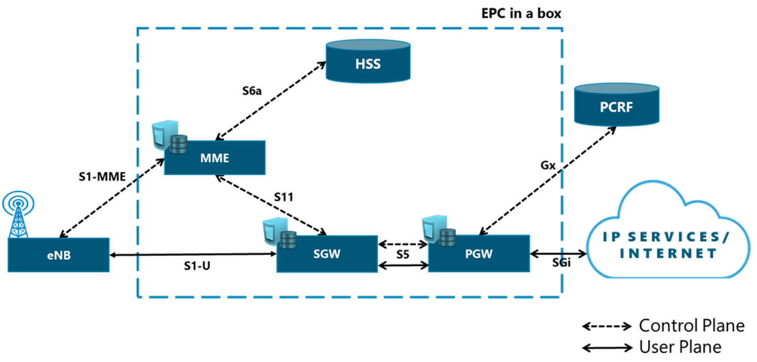
Figure 3. Evolved Packet Core Basic Architecture
The Mobile Core Architecture provides the overall EPC logical topology, the interconnection strategy with existing 2G/3G infrastructure and to external networks (e.g. Internet and other operators mobile core). From these inputs, the Mobile Core HLD Module defines the EPC minimum requirements related to Capacity Planning, VNF specifications, the networking protocol scheme and the redundancy mechanisms to assess from available solutions in the market appropriately.
The Mobile Core LLD spans through three main areas:
Firstly, the Bill of Materials (BoM) generation will be driven by the Bill of Quantities input from the HLD Module combined with the vendor information of the available solutions for the capacity dimensioning already calculated in the Mobile Core HLD Module.
Secondly, when the equipment from a vendor is already selected and the datasheets are shared with the NaaS Operator, the detailed diagrams of the physical and logical topologies can be drawn accurately referencing ports, hosts, logical external interfaces, protocol applicability, IPs and naming.
Finally, Mobile Core Low-Level Design (LLD) module aims to specify the key parameters of the selected protocols & virtualized solution. It also sets the parameters to the most commonly used values whenever possible in order to define a generic low-level design of the EPC solution.
2.1 Mobile Core LLD Environment
The main aspects to be considered when developing a low-level design of the Mobile Core are discussed in the following subsections:
Type of EPC Solution
The design process will vary according to the type of EPC solution. For core-in-a-box- solutions, they do not require such detailed information about the interconnection between EPC nodes, but only to external networks; they also do not need any IP planning or routing parameter definition for inside the box.
Some solutions require more complex configurations of specific services, performance enhancements and further customization, but these scenarios are out of scope of this module.
Network Function Virtualization Infrastructure (NFVI) Solution
The selection for using a virtualized solution was performed in the Mobile Core Architecture Module due to its advantages. The impact of implementing a virtualized solution on the overall process of the Mobile Core LLD module is as follows:
Management Strategy
The Management Strategy must have been defined in the Mobile Core Architecture Module. It includes the integration of BSS/OSS systems and the use of an Orchestration system for the virtualized elements. The impact of implementing an OSS/BSS system in the Mobile Core LLD process is as follows:
2.2 Mobile Core LLD Input Description
Identifying the most important inputs, there impact on the overall process and the possible sources is a key step towards an optimized and unambiguous LLD. The following table contains the inputs of the module along with their impact on the LLD process and potential sources:
|
Input Required |
Description |
Impact |
Source |
|
Mobile Core Architecture |
Architecture of the overall Mobile Core Solution, Service Definition and its required Network Elements. |
Architecture will drive the overall LLD. |
Mobile Core Architecture Module, Mobile Core HLD Module |
|
Roaming Strategy |
Roaming agreements with other MNOs and their approach to interconnection (Local breakout or Home routed). |
It will impact on the Routing and Switching Configuration, and IP Allocation and Assignment. |
Mobile Core Architecture Module |
|
Interconnection Requirements |
Existing infrastructure such as 2G/3G core networks, and strategy to interconnect to it (Gn/Gp or S3/S4 options). |
It will impact on the Routing and Switching Configuration, IP Allocation and Assignment and the Naming Convention and the Policy & Charging Rules Definition. |
Mobile Core Architecture Module, Mobile Core HLD Module, Existing Operator Data |
|
Operator Network Data |
Information related to existing infrastructure (Transport, RAN, Mobile Core), IP Pool availability and existing Naming Convention. |
Accurate information on existing networks will help Routing and Switching Configuration and Naming Convention. |
Operator Network Data, Existing Operator Network |
|
Redundancy Requirements |
High Availability Mechanisms to be integrated in the EPC. |
It will impact on the Routing and Switching Configuration, and IP Allocation and Assignment. |
Mobile Core HLD Module |
|
Bill of Quantities |
Document which contains the quantities of every logical entity/virtual network function. |
It will drive the Bill of Materials Generation. |
Mobile Core HLD Module |
Table 1. Mobile Core LLD Inputs
3 Functions & Methodologies
This section presents methodologies to perform critical tasks/subtasks involved in the Mobile Core design process.
3.1 IP Planning
The IP planning for a successful allocation, assignation and documentation must be defined according to the network requirements and appropriate granularity.
The first approach to the granularity is the division by service type: Network Foundation (i.e. all the routing protocols, switching and connection to the Internet); Network Services (i.e. features that operate in the background to improve and enable the user experience); and User Services (i.e. applications with which a user interacts directly such as voice, video, web surfing). Further subdivision may include the subdivision by plane, interface and location.
After the granularity is defined, the starting point will be selecting the IP address segment allocated for the Mobile Core elements. As seen on the Transport & IP Architecture Module, the IP range defined for the Mobile Core is 10.96.0.0/12. Within this segment, the needed subnets would be allocated by counting or estimating the number of IP addresses required.
According to the Transport & IP LLD Module, the steps towards an efficient IP planning are as follows:
For more detailed information, please refer to the corresponding module.
Step 1. Calculate the required block sizes
The elements that need an IP address are:
For example, if it is needed to design an IP planning for an EPC with the following characteristics:
The resulting subnet sizes will result from the operation of the number of elements multiplied for the number of IPs per element
For example, for Network Interface Connections:

To calculate the IP subnet masks, it is necessary to use the next formula (extracted from the Transport LLD Module):

(Eq. 1)
For example, for Network Interface Connections:
![]()
|
Category |
Subnet Purpose |
Number of required IP addresses |
Subnet Mask |
|
Hardware Infrastructure |
Network Interface Ports |
80 |
/25 |
|
Disk Array Controllers |
8 |
/29 |
|
|
Blades or computing hosts |
30 |
/27 |
|
|
Core Elements |
Loopback Interfaces |
20 |
/27 |
|
User Service Pool |
20,000 |
/17 |
Table 2 Summary of IP sizes per subnet
Step 2. Subnet Sorting
Sorting the subnets per mask size:
|
Subnet Purpose |
Number of required IP addresses |
Subnet Mask |
|
User Service Pool |
20,000 |
/17 |
|
Network Interface Ports |
80 |
/25 |
|
Blades or computing hosts |
30 |
/27 |
|
Loopback Interfaces |
20 |
/27 |
|
Disk Array Controllers |
8 |
/29 |
Table 3 Subnets sorted by network mask
Step 3. Subnets Assignment
The association with the assigned IP segment (10.96.0.0/12) is as follows:
|
Subnet Purpose |
Number of required IP addresses |
Subnet Mask |
|
User Service Pool |
20,000 |
10.96.0.0/17 |
|
Network Interface Ports |
80 |
10.96.128.0/25 |
|
Blades or computing hosts |
30 |
10.96.128.128/27 |
|
Loopback Interfaces |
20 |
10.96.128.160/27 |
|
Disk Array Controllers |
8 |
10.96.128.192/29 |
Table 4 Subnet assignation according to the IP segment
IP Planning widget can be used to ease the complexity of calculating the corresponding IP segments.
3.2 Routing and Switching Configuration
According to the Mobile Core HLD Module, a set of protocols can be used when configuring the routing and switching parts of the network.
For Layer 2, there is no option but to choose the Ethernet protocol. Furthermore, Virtual LANs (VLANs) can be implemented to separate traffic logically over the same Ethernet port (e.g logically separate O&M from the user/control traffic into a different VLAN). This is achieved by adding an ID (VLANs ID) to each Ethernet frame. It is recommended to allocate VLANs for specific purposes such as O&M, or EPC interfaces. The recommendation should look as follows:
For example, in the case that we have a number N of EPC interfaces coming out of one physical network port, it is necessary to segment the incoming/outgoing traffic by VLANs. In the case that all the O&M traffic is going out for one interface, the only VLAN associated with that specific physical network port is the VLAN associated with O&M purposes.
In terms of Layer 3, options of protocols include IGRP, EIGRP, OSPF and IS-IS for Interior Gateway Protocols, and BGP for Exterior Gateway Protocol. Although static routes are always an option for routing, it is recommended to use them only for a few scenarios, for example, when dealing with topologies that do not increase the quantity of network elements or connections over time.
Protocols to be implemented are previously defined in the Mobile Core HLD. The scope of the Low-Level Design is to provide the main parameters to be configured on Mobile Core nodes and routing equipment to support the defined protocols.
For layer 3 protocols configuration, the minimum parameters needed are:
The configuration must be done at the Mobile Core elements and the intermediate routing devices along the network. Although the commands for the routing protocols vary in syntax, the logic is the same: one Group ID may include several member interfaces and networks/subnetworks and these subnetworks will be able to communicate between them.
When the number of network/subnetworks is large (e.g., greater than 100), it is recommended to split them into smaller groups. In this way, the number of routing Group IDs will grow, but the routing information will not cause an overflood in the network. Routers or L3 switch can route between Group IDs if needed.
In a broader example, we may have the connection from one switch to one equipment as Figure 4:
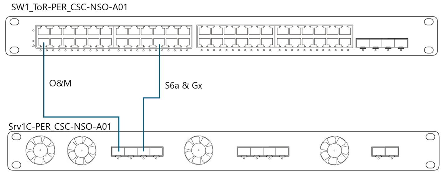
Figure 4. Example of interconnection from vEPC server 1 to Switch 1
In this case, the corresponding addresses for O&M, S6a and Gx EPC interfaces within the network segment for network interface ports from Table 4 (i.e. 10.96.128.0/25). The first subnetwork (10.96.128.0/30) should be tagged as VLAN 10 since this VLAN is assigned for O&M group of IPs. The second subnetwork (10.96.128.4/30) would be tagged as VLAN Group corresponding to S6a and Gx. The outgoing traffic would be tagged accordingly to the corresponding VLAN associated with the port. This concept can be applied to the scenario when multiple EPC interfaces are going out in one network interface port.
3.2.1 Security
Although network security is out of the scope of this module, general recommendations should be considered when implementing a vEPC solution and avoid future network security breaches.
Firstly, for overall network safety, an implementation of a firewall between the EPC and outer networks is strongly recommended. This firewall should be configured with Access Control Lists (ACL) to avoid unwanted traffic to go from the EPC to the external network and vice versa. These ACLs will also help to assure the isolation of traffic for different VLANs or network subnets that do not require to communicate with each other.
Secondly, it is also suggested to implement or configure features for Denial of Services attacks. These features are strongly advised to be integrated into the edge of the network, but they should also be configured between the EPC elements to strengthen the security.
Finally, routers and firewalls must be configured with rules to assure the isolation of traffic for different VLAN or network subnets that do not require to communicate to each other.
3.3 Diameter and GTP Configuration
Once the routing protocols are correctly configured, the work mode and parameters of Diameter and GTP protocols must be configured. The following subsections describe the logic to establish the configuration for each of these protocols.
3.3.1 GTP-based Interfaces
The GTP-based interfaces configuration consists of three steps:
Step 1. GTP binding
First, at every EPC network element, the GTP-based service must be bound to every logical IP address that will need to use GTP. There are two versions of this protocol (GTPv1 and GTPv2). GTPv2 is exclusively used for Control Plane whereas GTPv1 for User Plane. If one interface carries both planes, it must be bound to both versions.
Step 2. NAPTR Records Definition
The second step is to define the NAPTR records for establishing communication between network elements using GTP interfaces. The NaaS operator must perform this process for every interface that needs to support GTP.
For GTP connections there is no auto-discovery method and it must be defined as a Domain Name Service (DNS) record with compliance to 3GPP standard TS 23.003. The format for these records must be a Name Authority Pointer (NAPTR). The NAPTR format components for EPC includes the service and the node information.
The NaaS operator must define a DNS record for every Mobile Core element with at least one GTP interface. These records are consulted to know the IP address of the required equipment interface. The list of the components and its description can be found in Table 5.
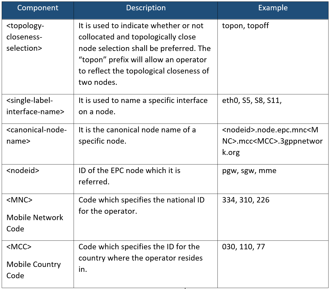
Table 5 Components of NAPTR Records for EPC elements
The NAPTR DNS records are always mapped to an IP address or a set of IP addresses which are contained in the DNS Server. Although it is strongly advisable to have a DNS server with records for inner EPC GTP interfaces, it is not strictly necessary as these can be configured locally on every equipment and not depending on an external device.
A sample record is shown below:
topoff.s8.pgw.node.epc.mnc030.mcc310.3gppnetwork.org
Analyzing the sample record, it refers to a node that is not eligible for closeness selection (topoff), this could be used for roaming interfaces (S8) where the connection from a Home SGW to Visitor PGW is needed (pgw). It also indicates that it is a node from the EPC core whose MNC and MCC are 030 and 310.
Step 3. NAPTR Records Configuration
As the last step, it is needed to configure a default GTP pair at every interface. Once the configuration is done, EPC elements can communicate with each other by asking the DNS Server to resolve the NAPTR records and retrieve the corresponding IP address.
For example, the S11 interface on one MME needs to communicate with the S11 interface of one SGW. The DNS records defined are as follows:
On the MME a default rule will be configured with the indication that all the signaling must go to the SGW:
For ALL_USERS the S11_INTERFACE is topoff.s11.sgw.node.epc.mnc030.mcc310.3gppnetwork. org.
The MME should look into the configured DNS server and retrieve the IP(s) for reaching its counterpart in the SGW.
NAPRT Record widget can be used to avoid error when generating NAPTR records for GTP Interfaces.
3.3.2 Diameter-based Interfaces
For Diameter-based interfaces, the roaming and local nodes are equally treated and do not require any special configuration. Diameter protocol only needs the following parameters on both ends:
In the following example, a PCRF and a PGW want to connect through the Gx interface. The PGW must initialize the communication to the PCRF as the latter only listens to requests. The chosen transport mechanism is SCTP over the default port (3868). Table 6 displays the information elements for the aforementioned example:
|
Endpoint 1 (PCRF) |
Endpoint 2 (PGW) |
||
|
Hostname |
pcrf.gx.operator |
pgw.gx.operator |
|
|
IP address and format |
10.99.0.1/32 (IPv4) |
10.100.0.1/32 (IPv4) |
|
|
Port |
3868 |
||
|
Work Mode |
Listen |
Initialize + Listen |
|
|
Transport Protocol |
SCTP |
||
|
Supported Applications |
16777238: Gx |
||
Table 6 Example of required Information of Diameter endpoints
The following steps must be followed to configure the Diameter protocol in the example:
3.4 Policy and Charging Rules Logical Design
The Policy and Charging Rules logical design should be based on the level of granularity for the operator business and service model. Examples of these models are the different thresholds for data consumption, voice time budget and VoLTE or another enhanced functionality; all of which lead to wider subscription plans available to address the final user needs.
The logical design contemplates the use of criteria and thresholds which triggers a set of specific and well-identified actions. The most known behavior is for data consumption. When a user consumes a certain amount of data, the service is interrupted and the user is redirected to a captive portal for buying more credit balance. It is important to know that other actions can be applied together such as QoS/Bit Rate degradation or charging rate modification.
This guide only attempts to provide the main criteria on what kind of actions and rules can be logically implemented in order to have a complete ecosystem for charging and policy ruling. Table 7 contains these criteria, its descriptions and possible actions to be taken by the Mobile Cores Policy and Charging Enforcement Function (PCEF):
|
Criteria |
Description |
Possible Actions |
|
Data Usage Consumption |
Given the credit balance measurement and once reached its limit, the service is modified |
Bit Rate modification, data service interruption, QoS Modification. |
|
Roaming Restriction |
The UE enters in roaming scenarios |
Bit Rate modification, specific service interruption, charging rate modification. |
|
IMS Profiling |
Special case as the VoLTE users need a dedicated bearer establishment when making phone calls. |
Establishment of the dedicated bearer, QoS modification. |
|
Modified QoS |
Modification to QoS based on location, emergency scenarios or services. |
Downgrade or upgrade of QoS index associated with a service. |
|
Bit Rate Modification |
The UE may have reached a limit in a service, it is upgraded to a better plan or dimension adjustments. |
Downgrade or upgrade of Bit Rate. |
|
Location-Based Charging |
Charging rates based on the location of the UE. |
Increase or decrease in certain locations. |
|
Differentiated Charging |
A change in charging rates when specific conditions are met. |
The charging rate is elevated or decreased. |
|
Specific Service |
A specific service triggers action(s). |
Bit Rate modification, charging rate modification, establishment of a dedicated bearer or QoS modification |
Table 7 Common Policy and Charging Rule Logic Criteria
Either the operator would choose some of the directives, a combination of them or none. As an example, we can assume that two criteria were selected for one user:
If the user reaches its data consumption, it will continue its web surfing at a reduced bit rate. If the same user reaches its data consumption when roaming, the service will be interrupted. In conclusion, for the same criteria, different actions may take place depending on the scenario and associated rules.
The final format should be a spreadsheet with all the rules and associated actions that later can be easily translated into CLI if necessary. The previous example should look as Table 8:
|
Criteria |
Threshold |
Action(s) |
|
Data Usage Consumption |
2 GB |
Bit Rate Degradation 1 Mbps -> 128 kbps |
|
Roaming Restriction |
Connected to a Roaming network |
Bit Rate Degradation 1 Mbps -> 512 kbps |
|
Data Usage Consumption + Roaming Restriction |
2 GB + Connected to a Roaming network |
Complete service interruption + Redirection to the captive portal |
Table 8. Policy and Charging Rule Format Example
It is important to mention that the real-time billing is responsibility of the Online Charging System (OCS), whereas the policy and charging rules are contained in the PCRF and the final actions are applied by the PCEF (often included in the PGW logical entity).
4 E2E Process Flow
Generic yet customizable end-to-end process flow to perform the design for the mobile core network.
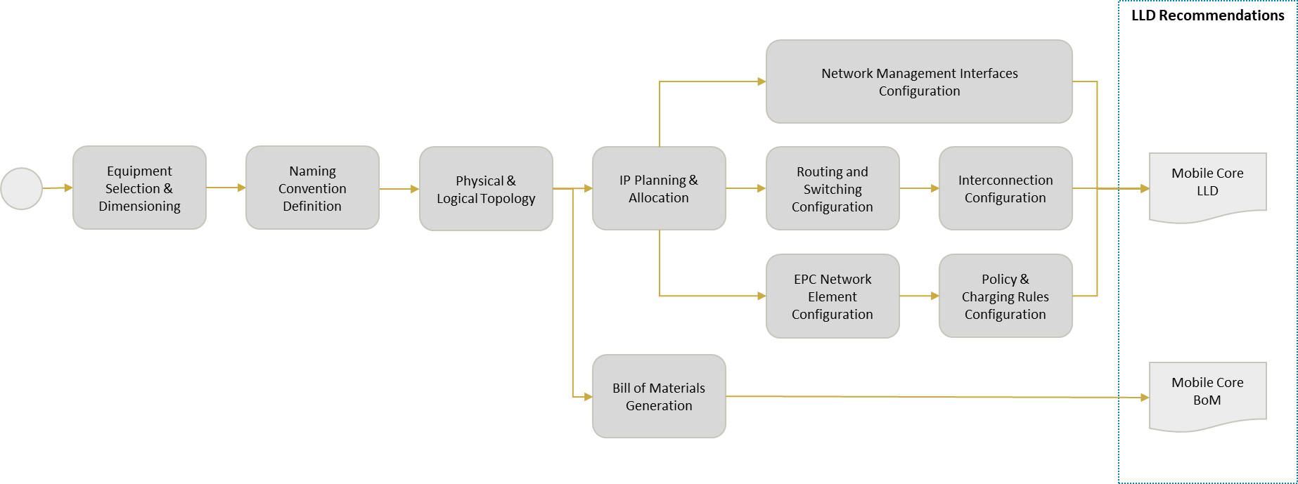
Figure 5. Mobile Core LLD Design Process
4.1 End-to-end Process Overview
As presented in Figure 5, the end-to-end process consists of eleven main steps. Each step has some dependencies and necessary inputs, which are addressed in the corresponding section.
The first step is Equipment Selection and Dimensioning, which consists of the appropriate selection of the VNFs and virtualized solution that best covers the requirements from the Capacity Planning done in the Mobile Core HLD Module. The Naming Convention is a set of rules for defining a proper identification for every element in the network, which includes operator and logical entities information.
The third and fourth phases are Hardware Description Layout and Physical and Logical Topology, which are diagrams that detail the physical equipment, connections to other physical equipment and the logical interconnection of the whole network.
The IP Planning and Allocation, the Routing and Switching Configuration and the Interconnection Configuration allows the design for the networking stage to properly communicate between inner EPC nodes and to external networks. It includes the most common parameters needed to be configured, from IP allocation to GTP and Diameter Protocols parameters.
The Network Management Interfaces Configuration provides directives for configuring the Operation and Maintenance (O&M) interfaces to OSS/BSS centralized systems.
The EPC Network Element Configuration provides the guidance for the configuration of basic parameters in each logical node of the EPC. Policy & Charging Rules Configuration describes the key elements for designing rules that can modify the users and services parameters (e.g. differentiated QoS or Charging Rates).
Finally, the Bill of Materials generation is described, based on the outputs of the module, which will serve as the principal input for the Purchase Order Generation.
4.2 Step-by-step Analysis
In order to demonstrate a practical exercise to implement the process design flow, a Design Example is developed along with each of the process steps. Before getting into the details of the process, an overview of the design example scenario is presented.
Design Example: Scenario Definition
In this particular example, the process to generate the LLD Design is presented for the scenario shown in the following figure, which corresponds to a Roaming scenario. It is important to note that it has the same characteristics that the example in Mobile Core HLD.
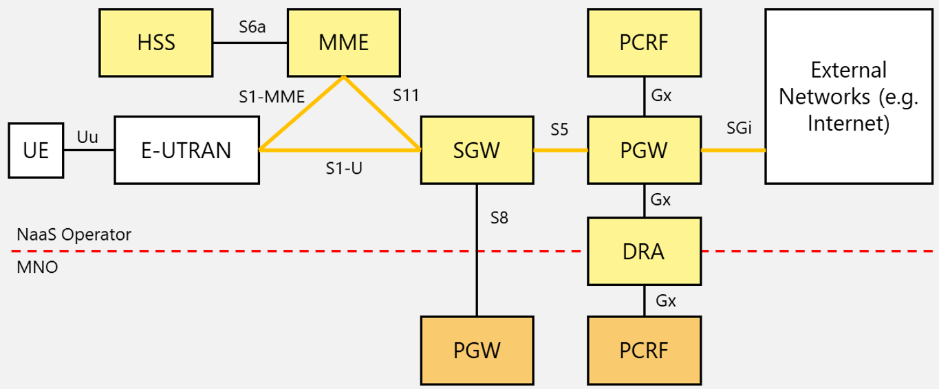
Capacity Planning Requirements:
– 650k total users
– 260k Simultaneously Attached Users
– 10 Gbps maximum throughput
– Mandatory Redundancy at Server Level 1+1 in Standby Mode
– Information provided from vendors is shown below. In this case, the virtualized EPC solution is provided as a VNF bundle.
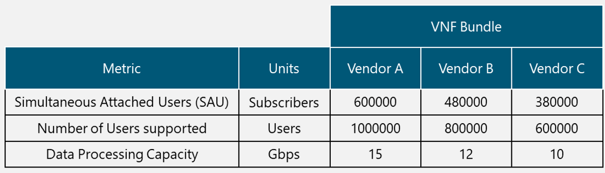
The hardware requirements for each VNF Bundle are as follows:
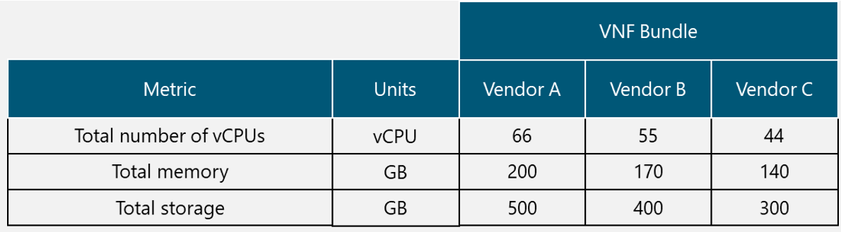
The hardware solutions that instantiate the virtualized EPC supported by each vendor are:
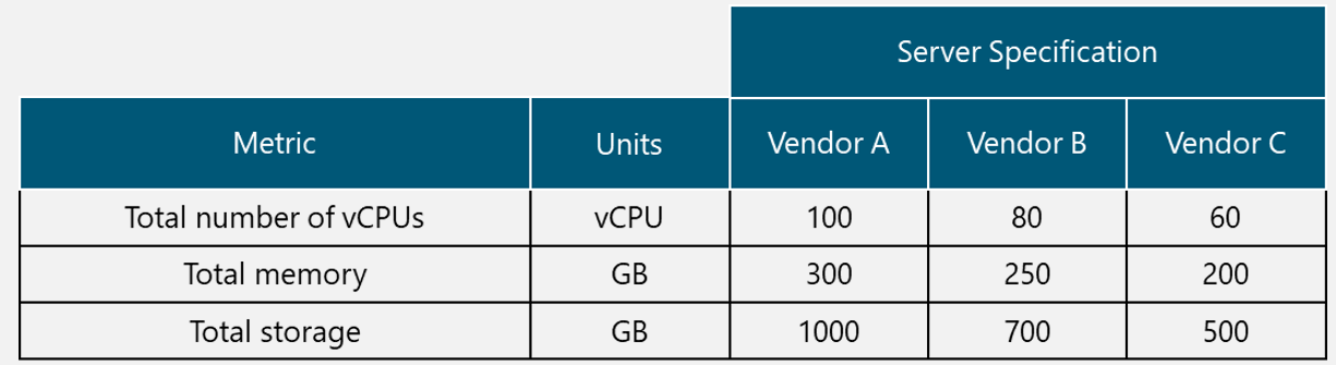
The segment 10.96.0.0/11 has been allocated by the Tx & IP Architecture module for the Mobile Core elements.
Operator Data:
– Mobile Network Code (MNC): 33
– Mobile Country Code (MCC): 610
– Country Code (CC): 86
– NTP Server info: server 0.north-america.pool.ntp.org
EPC Data defined by operator:
– MME Group ID: 3000
– MME Code: 1
– Default APN: internet.NaaS.com
– User Default Profile: Data Service, 50000 kbps AMBR, Best Effort QoS (QCI9), using default APN
4.2.1 Equipment Selection & Dimensioning
The Equipment Selection and Dimensioning process is presented as a first step in every EPC implementation. It has a dependency on the Bill of Quantities and the Capacity Planning outputs from the Mobile Core HLD Module.
This process basically consists of two main steps:
The VNFs can be offered as a group to cover several NEs, which can be identified as VNF Bundle.
The selection of the VNF Bundle can be done once the Request for Information (RFI) phase is already finished. The approach for this selection must be based on metrics from Capacity Planning for which the equipment selection must cover successfully all of them (e.g. maximum number of subscribers, simultaneous attached users, simultaneous active sessions, transactions per second, services or features).
The next formula, taken from Mobile Core HLD Module, applies also for the Virtual Network Function (VNF) dimensioning:

(Eq. 3)
The VNF quantity (![]() ) is given by the relation of all the calculated metrics per NE (
) is given by the relation of all the calculated metrics per NE (![]() ) mapped to its corresponding VNF capacity metric (
) mapped to its corresponding VNF capacity metric (![]() ), rounded up and selecting the larger value, which indicates the total amount of VNFs. If the VNF has the capability for handling more than one Network Element (NE), it must cover the metrics for all the NEs contained.
), rounded up and selecting the larger value, which indicates the total amount of VNFs. If the VNF has the capability for handling more than one Network Element (NE), it must cover the metrics for all the NEs contained.
The second step is the dimensioning phase to map the requirements of those VNF Bundles into hardware requirements. The procedure would be similar since the principle is the same: calculate the equipment that covers all the requirements for the required VNFs.
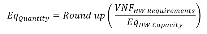
(Eq. 4)
The equipment, with hardware capacity (![]() ) (e.g vCPUs, memory or storage capacity), that best covers all the metrics for the VNFs (
) (e.g vCPUs, memory or storage capacity), that best covers all the metrics for the VNFs (![]() ) without the need for more than one physical equipment (
) without the need for more than one physical equipment (![]() ) would be the ideal solution. This will avoid the dependency on large number of interconnections and ease the complexity of the network.
) would be the ideal solution. This will avoid the dependency on large number of interconnections and ease the complexity of the network.
Design Example
VNF Bundle Quantity:
According to Eq (1), the number of VNF bundles can be calculated for each of their different metrics and picking up the maximum value rounded up.
– 650k total users
– 260k Simultaneous Attached Users
– 10 Gbps maximum throughput
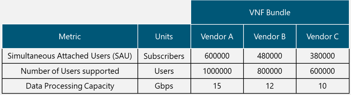
For Vendor A:
![]()
For Vendor B:
![]()
For Vendor C:
![]()
It is clear that the two possible solutions that cover all the metrics are from Vendor A and B since both only need one VNF bundle. However, the solution from Vendor B will be selected as it has less overcapacity and consequently requires less hardware.

According to the previous table, the requirements for this solution are: 55 vCPU, 170 GB RAM Memory and 400 GB Storage.
Equipment Quantity:
The equipment from the same vendors have the following characteristics:
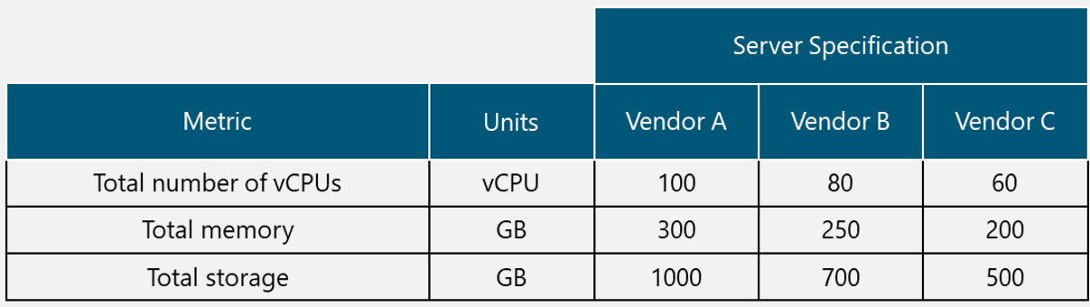
There are several considerations when selecting a Server Infrastructure:
– Total price (cheapest is best)
– Overcapacity (less idle capacity is best)
– Number of servers (less is best)
To cope with the hardware requirements for VNF Bundle from vendor B, is it necessary 55 vCPU, 170 GB RAM Memory and 400 GB Storage. It is clear that server specifications from vendor A and vendor B cover the hardware requirements with just one server whereas two servers from vendor C are needed for the same purpose.
– Total Price: Vendor C can be an option if the total price of the two servers is less than the other options (one server from vendor A or one server from vendor B).
– Overcapacity: Vendor B is the option with less overcapacity compared to Vendor A and two servers from Vendor C.
– Number of servers: Since the server infrastructure from the vendors can consist of several server units, the server infrastructure with a smaller number of servers can be a decision point if previous considerations have not done a clear selection yet.
In this example, the total price from vendor C is cheaper than the other options even though it consists of two separate servers. The solution from vendor C has a greater idle hardware resource, but they can be used when forecasted capacity analysis is carried out.
In conclusion, the VNF Bundle from Vendor B and two server infrastructures from Vendor C will be selected.
4.2.2 Naming Convention Definition
The naming convention is always part of the LLD process since all the physical and logical equipment has to be named in order to be easily identified in the network.
The naming convention process is the only one that has almost a total independence from any other process. It can be performed at any point in the design without affecting other processes outputs. However, it is recommended to be performed before the IP planning step for a better organization and clarity.
In case there is not a pre-existing naming convention, the following recommendations should be followed by the NaaS operator. First, it has to be unique in the entire private network, it must contain elements that do not change over time and are easy to understand, but it does not have to be so long nor too complex.
Despite the complexity of the network, the name at least has to comply with the aspects on Table 9 to differentiate the equipment effectively.
|
Type |
Description |
Example |
|
Entity |
The name of the physical/logical equipment, entity or interface. This is the only field that can vary in length. In the case of interfaces, it can contain 2 Entity fields. |
MME, SGW, PGW, HSS, S1-MME, S8, |
|
Location |
Given the name of the location. |
DEN, CAL, NYC, CSC |
|
Operator Info |
The name of the NaaS Operator is the minimum information that must be included. |
NSO, IpT, MMA |
|
Unique ID |
A unique identifier can be included at the end of the name to avoid duplicity. |
A1, B01, 01 |
Table 9 Basic naming components for Mobile Core Elements
It is a good practice to keep the names elements as short as possible without making it ambiguous; three letters per field may suffice. Although separators such as hyphens, underscores or dots help to make it clear and easy to understand, they could not be supported for every equipment and it must be verified beforehand. Special characters should not be used in order to avoid ambiguities and/or language typing dependencies. It is important to consider the equipment constraints on the allowed characters and the maximum length.
Another good practice is to detail what the elements of the naming convention are and its description along with some notes of the meaning of the abbreviations.
Naming convention widget can be used for simplify this step.
Design Example
Naming Convention:
In this example, the elements are positioned in priority order so the union of the elements will give a complete name of the element:
(Entity name)-(Country)_(Location)-(NaaS Operator Name)-(Unique ID)
For example:
MME-PER_CSC-NSO-A01
The name itself indicates that we are talking about an MME located in Cusco, Peru, that belongs to NaaS Operator Network with unique identifier A01 in case there are more similar equipment in the same installation.
4.2.3 Physical and Logical Topology
The physical and logical topology process is needed for every implementation of the Mobile Core, no matter what kind of solution it addresses. This step defines the logical and physical connections required to comply with the architectures design; it takes as inputs the following:
The first step is to map the logical entities (e.g. network elements and core interfaces) to the physical hardware in a table form. This allows the NaaS to have a better understanding of how logical connections will drive the physical ones. The parameters needed for the table are: names of the logical and physical elements (in case of interfaces both ends of the interface or ports) according to the naming convention process.
Table 11 displays an example of Server A, which contains all the EPC core elements and includes a switch Top of Rack A (ToR) that uses three ports to divide the traffic into O&M+Sync, Control Plane (CP) and User Plane (UP). As a redundancy, it is included a Server B with the same EPC elements connected to the same switch ToR. It is important to note that, for this example, only interfaces for external network connections are included in these outwards physical ports. If more than one server is implemented due to the selected solution or due to redundancy mechanisms, they all must be named accordingly.
|
Logical Element |
|
|
Name of the Server A (SrvA) |
MME1, SGW1, PGW1, HSS1, |
|
Name of the Server B for redundancy (SrvB) |
MME1, SGW1, PGW1, HSS1 (Same EPC elements since it is under standby scheme) |
|
SwitchA_TOR_Port0/0 |
All O&M & Sync |
|
SwitchA_TOR_Port0/1 |
S8 (CP), S1-MME |
|
SwitchA_TOR_Port0/2 |
S1-U, S8 (UP), SGi |
|
SwitchA_TOR_Port0/3 |
All O&M & Sync (Redundant) |
|
SwitchA_TOR_Port0/4 |
S8 (CP), S1-MME (Redundant) |
|
SwitchA_TOR_Port0/5 |
S1-U, S8 (UP), SGi (Redundant) |
Table 11. Mapping table for Hardware-to-Logical Elements
As a second step, once identified the logical to physical equipment, the connections between them are drawn according to data on the table. There are two types of output diagrams for this step: logical and physical.
Design Example
Physical and Logical Topology:
The logical diagram considering the NFV solution for the whole EPC nodes:
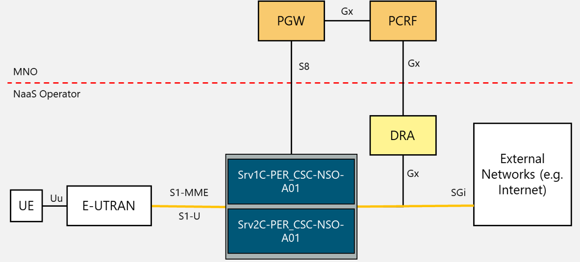
The VNF distribution could be:
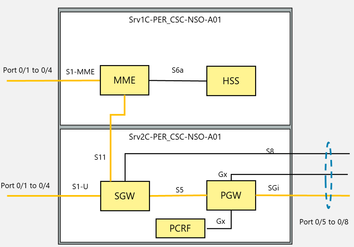
|
Hardware Element |
Logical Element |
|
Srv1C-PER_CSC-NSO-A01 |
MME, HSS |
|
Srv2C-PER_CSC-NSO-A01 |
SGW, PGW |
|
Srv1C-PER_CSC-NSO-B01 (Standby) |
MME, HSS |
|
Srv2C-PER_CSC-NSO-B01 (Standby) |
SGW, PGW |
|
Srv1C-PER_CSC-NSO-A01 Port 0/1 Srv1C-PER_CSC-NSO-A01 Port 0/2 Srv1C-PER_CSC-NSO-A01 Port 0/3 Srv1C-PER_CSC-NSO-A01 Port 0/4 |
S1-MME |
|
Srv1C-PER_CSC-NSO-A01 Port 0/5 Srv1C-PER_CSC-NSO-A01 Port 0/6 Srv1C-PER_CSC-NSO-A01 Port 0/7 Srv1C-PER_CSC-NSO-A01 Port 0/8 |
Reserved |
|
Srv2C-PER_CSC-NSO-A01 Port 0/1 Srv2C-PER_CSC-NSO-A01 Port 0/2 Srv2C-PER_CSC-NSO-A01 Port 0/3 Srv2C-PER_CSC-NSO-A01 Port 0/4 |
S1-U |
|
Srv2C-PER_CSC-NSO-A01 Port 0/5 Srv2C-PER_CSC-NSO-A01 Port 0/6 Srv2C-PER_CSC-NSO-A01 Port 0/7 Srv2C-PER_CSC-NSO-A01 Port 0/8 |
Gx, S8 & SGi |
|
Srv1C-PER_CSC-NSO-B01 Port 0/1 Srv1C-PER_CSC-NSO- B01 Port 0/2 Srv1C-PER_CSC-NSO- B01 Port 0/3 Srv1C-PER_CSC-NSO- B01 Port 0/4 |
S1-MME (Standby) |
|
Srv2C-PER_CSC-NSO- B01 Port 0/1 Srv2C-PER_CSC-NSO- B01 Port 0/2 Srv2C-PER_CSC-NSO- B01 Port 0/3 Srv2C-PER_CSC-NSO- B01 Port 0/4 |
S1-U (Standby) |
|
Srv2C-PER_CSC-NSO- B01 Port 0/5 Srv2C-PER_CSC-NSO- B01 Port 0/6 Srv2C-PER_CSC-NSO- B01 Port 0/7 Srv2C-PER_CSC-NSO- B01 Port 0/8 |
Gx, S8 & SGi (Standby) |
|
Srv2C-PER_CSC-NSO- B01 Port 0/5 Srv2C-PER_CSC-NSO- B01 Port 0/6 Srv2C-PER_CSC-NSO- B01 Port 0/7 Srv2C-PER_CSC-NSO- B01 Port 0/8 |
Reserved (Standby) |
For the interconnection to external networks, the connection is done through a layer 3 switch which was identified as SW1_ToR-PER_CSC-NSO-A01 according to the naming convention. The links were designed as follows:
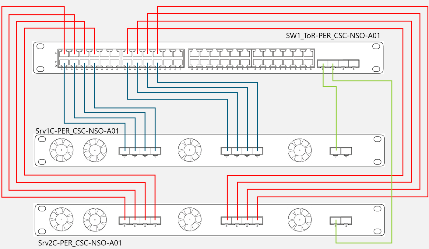
The blue links are corresponding to the Server 1 to Switch ToR 1 whereas the red links go from server 2 to Switch ToR 1, all these links correspond to 10 Gigabit Ethernet. On the other hand the green links correspond to 1 GE for O&M purposes. It is important to remark that this diagram can be used for the redundancy, but the connection from switch to switch for intercommunication between servers are as follows:
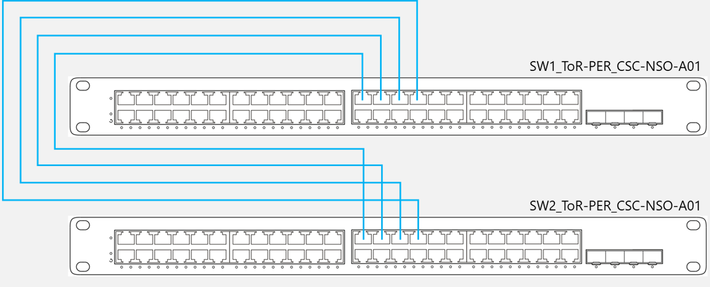
In this diagram, the blue lines indicate the links from Switch ToR 1 to Switch ToR 2
|
Device A |
Device B |
Link Type |
|
Srv1C-PER_CSC-NSO-A01 (Port 0/1) |
SW1_ToR-PER_CSC-NSO-A01 (Port 1/1) |
10 GE |
|
Srv1C-PER_CSC-NSO-A01 (Port 0/2) |
SW1_ToR-PER_CSC-NSO-A01 (Port 1/2) |
10 GE |
|
Srv1C-PER_CSC-NSO-A01 (Port 0/3) |
SW1_ToR-PER_CSC-NSO-A01 (Port 1/3) |
10 GE |
|
Srv1C-PER_CSC-NSO-A01 (Port 0/4) |
SW1_ToR-PER_CSC-NSO-A01 (Port 1/4) |
10 GE |
|
Srv1C-PER_CSC-NSO-A01 (Port 0/5) |
SW1_ToR-PER_CSC-NSO-A01 (Port 1/7) |
10 GE |
|
Srv1C-PER_CSC-NSO-A01 (Port 0/6) |
SW1_ToR-PER_CSC-NSO-A01 (Port 1/8) |
10 GE |
|
Srv1C-PER_CSC-NSO-A01 (Port 0/7) |
SW1_ToR-PER_CSC-NSO-A01 (Port 1/9) |
10 GE |
|
Srv1C-PER_CSC-NSO-A01 (Port 0/8) |
SW1_ToR-PER_CSC-NSO-A01 (Port 1/10) |
10 GE |
|
Srv1C-PER_CSC-NSO-A01 (Port 1/1) |
SW1_ToR-PER_CSC-NSO-A01 (Port 2/1) |
1 GE |
|
Srv2C-PER_CSC-NSO-A01 (Port 0/1) |
SW1_ToR-PER_CSC-NSO-A01 (Port 0/1) |
10 GE |
|
Srv2C-PER_CSC-NSO-A01 (Port 0/2) |
SW1_ToR-PER_CSC-NSO-A01 (Port 0/2) |
10 GE |
|
Srv2C-PER_CSC-NSO-A01 (Port 0/3) |
SW1_ToR-PER_CSC-NSO-A01 (Port 0/3) |
10 GE |
|
Srv2C-PER_CSC-NSO-A01 (Port 0/4) |
SW1_ToR-PER_CSC-NSO-A01 (Port 0/4) |
10 GE |
|
Srv2C-PER_CSC-NSO-A01 (Port 0/5) |
SW1_ToR-PER_CSC-NSO-A01 (Port 0/7) |
10 GE |
|
Srv2C-PER_CSC-NSO-A01 (Port 0/6) |
SW1_ToR-PER_CSC-NSO-A01 (Port 0/8) |
10 GE |
|
Srv2C-PER_CSC-NSO-A01 (Port 0/7) |
SW1_ToR-PER_CSC-NSO-A01 (Port 0/9) |
10 GE |
|
Srv2C-PER_CSC-NSO-A01 (Port 0/8) |
SW1_ToR-PER_CSC-NSO-A01 (Port 0/10) |
10 GE |
|
Srv2C-PER_CSC-NSO-A01 (Port 1/1) |
SW1_ToR-PER_CSC-NSO-A01 (Port 2/2) |
1 GE |
|
SW1_ToR-PER_CSC-NSO-A01 (Port 0/13) |
SW2_ToR-PER_CSC-NSO-A01 (Port 0/13) |
10 GE |
|
SW1_ToR-PER_CSC-NSO-A01 (Port 0/14) |
SW2_ToR-PER_CSC-NSO-A01 (Port 0/14) |
10 GE |
|
SW1_ToR-PER_CSC-NSO-A01 (Port 0/15) |
SW2_ToR-PER_CSC-NSO-A01 (Port 0/15) |
10 GE |
|
SW1_ToR-PER_CSC-NSO-A01 (Port 0/16) |
SW2_ToR-PER_CSC-NSO-A01 (Port 0/16) |
10 GE |
4.2.4 IP Planning & Allocation
The allocation of IPs must be done according to the logical entities that are planned to be included in the network topology. After the VNF and NFVI dimensioning, a good estimation of the number of required IP addresses can be made. Please refer to section 3.1 for the details of what elements of the topology needs an IP segment and their respective sizes.
The IP Planning process needs the output from several phases. The most important characteristic from each step is: logical and physical equipment quantity from Equipment Dimensioning; redundancy granularity from Redundancy Assessment; and the whole format identifiers from Naming Convention.
After this process, the summarization of all the subnets is necessary and can be consulted in the Tx and IP Design Module.
Design Example
IP Planning and Allocation:
The quantities are as follows for this example:
Hardware Infrastructure
o 40 Network Interface connections
o 8 disk array controllers (assuming 4 disk arrays, 2 controllers per array)
o 30 computing hosts
Logical Elements
o 30 loopback interfaces
o 260k simultaneous active sessions (Data Only, 1 bearer per active user)
Step 1. Calculate the required block sizes
|
Category |
Subnet Purpose |
Number of required IP addresses |
Subnet Mask |
|
Hardware Infrastructure |
Network Interface Ports |
160 |
/24 |
|
Disk Array Controllers |
8 |
/28 |
|
|
Blades or computing hosts |
30 |
/26 |
|
|
Core Elements |
Loopback Interfaces |
30 |
/26 |
|
User Service Pool |
260,000 |
/14 |
Step 2. Subnet Sorting
|
Subnet Purpose |
Number of required IP addresses |
Subnet Mask |
|
User Service Pool |
260,000 |
/14 |
|
Network Interface Ports |
160 |
/24 |
|
Blades or computing hosts |
30 |
/26 |
|
Loopback Interfaces |
30 |
/26 |
|
Disk Array Controllers |
8 |
/28 |
Step 3. Subnets Assignment
|
Subnet Purpose |
Number of required IP addresses |
Subnet Mask |
|
User Service Pool |
260,000 |
10.96.0.0/14 |
|
Network Interface Ports |
160 |
10.100.0.0/24 |
|
Blades or computing hosts |
30 |
10.101.0.0/26 |
|
Loopback Interfaces |
30 |
10.101.64.0/26 |
|
Disk Array Controllers |
8 |
10.101.128.0/28 |
For example, for physical ports connections the IP distribution would look like:
|
Device A |
Device B |
Network |
|
Srv1C-PER_CSC-NSO-A01 (Port 0/1) |
SW1_ToR-PER_CSC-NSO-A01 (Port 1/1) |
10.100.0.0/30 |
|
Srv1C-PER_CSC-NSO-A01 (Port 0/2) |
SW1_ToR-PER_CSC-NSO-A01 (Port 1/2) |
10.100.0.4/30 |
|
Srv1C-PER_CSC-NSO-A01 (Port 0/3) |
SW1_ToR-PER_CSC-NSO-A01 (Port 1/3) |
10.100.0.8/30 |
|
Srv1C-PER_CSC-NSO-A01 (Port 0/4) |
SW1_ToR-PER_CSC-NSO-A01 (Port 1/4) |
10.100.0.12/30 |
|
Srv1C-PER_CSC-NSO-A01 (Port 0/5) |
SW1_ToR-PER_CSC-NSO-A01 (Port 1/7) |
10.100.0.16/30 |
|
Srv1C-PER_CSC-NSO-A01 (Port 0/6) |
SW1_ToR-PER_CSC-NSO-A01 (Port 1/8) |
10.100.0.20/30 |
|
Srv1C-PER_CSC-NSO-A01 (Port 0/7) |
SW1_ToR-PER_CSC-NSO-A01 (Port 1/9) |
10.100.0.24/30 |
|
Srv1C-PER_CSC-NSO-A01 (Port 0/8) |
SW1_ToR-PER_CSC-NSO-A01 (Port 1/10) |
10.100.0.28/30 |
|
Srv1C-PER_CSC-NSO-A01 (Port 1/1) |
SW1_ToR-PER_CSC-NSO-A01 (Port 2/1) |
10.100.0.32/30 |
|
Srv2C-PER_CSC-NSO-A01 (Port 0/1) |
SW1_ToR-PER_CSC-NSO-A01 (Port 0/1) |
10.100.0.36/30 |
|
Srv2C-PER_CSC-NSO-A01 (Port 0/2) |
SW1_ToR-PER_CSC-NSO-A01 (Port 0/2) |
10.100.0.40/30 |
|
Srv2C-PER_CSC-NSO-A01 (Port 0/3) |
SW1_ToR-PER_CSC-NSO-A01 (Port 0/3) |
10.100.0.44/30 |
|
Srv2C-PER_CSC-NSO-A01 (Port 0/4) |
SW1_ToR-PER_CSC-NSO-A01 (Port 0/4) |
10.100.0.48/30 |
|
Srv2C-PER_CSC-NSO-A01 (Port 0/5) |
SW1_ToR-PER_CSC-NSO-A01 (Port 0/7) |
10.100.0.52/30 |
|
Srv2C-PER_CSC-NSO-A01 (Port 0/6) |
SW1_ToR-PER_CSC-NSO-A01 (Port 0/8) |
10.100.0.56/30 |
|
Srv2C-PER_CSC-NSO-A01 (Port 0/7) |
SW1_ToR-PER_CSC-NSO-A01 (Port 0/9) |
10.100.0.60/30 |
|
Srv2C-PER_CSC-NSO-A01 (Port 0/8) |
SW1_ToR-PER_CSC-NSO-A01 (Port 0/10) |
10.100.0.64/30 |
|
Srv2C-PER_CSC-NSO-A01 (Port 1/1) |
SW1_ToR-PER_CSC-NSO-A01 (Port 2/2) |
10.100.0.68/30 |
|
Srv1C-PER_CSC-NSO-B01 (Port 0/1) |
SW2_ToR-PER_CSC-NSO-A01 (Port 1/1) |
10.100.0.72/30 |
|
Srv1C-PER_CSC-NSO-B01 (Port 0/2) |
SW2_ToR-PER_CSC-NSO-A01 (Port 1/2) |
10.100.0.76/30 |
|
Srv1C-PER_CSC-NSO-B01 (Port 0/3) |
SW2_ToR-PER_CSC-NSO-A01 (Port 1/3) |
10.100.0.80/30 |
|
Srv1C-PER_CSC-NSO-A01 (Port 0/4) |
SW2_ToR-PER_CSC-NSO-A01 (Port 1/4) |
10.100.0.84/30 |
|
Srv1C-PER_CSC-NSO-B01 (Port 0/5) |
SW2_ToR-PER_CSC-NSO-A01 (Port 1/7) |
10.100.0.88/30 |
|
Srv1C-PER_CSC-NSO-B01 (Port 0/6) |
SW2_ToR-PER_CSC-NSO-A01 (Port 1/8) |
10.100.0.92/30 |
|
Srv1C-PER_CSC-NSO-B01 (Port 0/7) |
SW2_ToR-PER_CSC-NSO-A01 (Port 1/9) |
10.100.0.96/30 |
|
Srv1C-PER_CSC-NSO-B01 (Port 0/8) |
SW2_ToR-PER_CSC-NSO-A01 (Port 1/10) |
10.100.0.100/30 |
|
Srv1C-PER_CSC-NSO-B01 (Port 1/1) |
SW2_ToR-PER_CSC-NSO-A01 (Port 2/1) |
10.100.0.104/30 |
|
Srv2C-PER_CSC-NSO-B01 (Port 0/1) |
SW2_ToR-PER_CSC-NSO-A01 (Port 0/1) |
10.100.0.108/30 |
|
Srv2C-PER_CSC-NSO-B01 (Port 0/2) |
SW2_ToR-PER_CSC-NSO-A01 (Port 0/2) |
10.100.0.112/30 |
|
Srv2C-PER_CSC-NSO-B01 (Port 0/3) |
SW2_ToR-PER_CSC-NSO-A01 (Port 0/3) |
10.100.0.116/30 |
|
Srv2C-PER_CSC-NSO-B01 (Port 0/4) |
SW2_ToR-PER_CSC-NSO-A01 (Port 0/4) |
10.100.0.120/30 |
|
Srv2C-PER_CSC-NSO-B01 (Port 0/5) |
SW2_ToR-PER_CSC-NSO-A01 (Port 0/7) |
10.100.0.124/30 |
|
Srv2C-PER_CSC-NSO-B01 (Port 0/6) |
SW2_ToR-PER_CSC-NSO-A01 (Port 0/8) |
10.100.0.128/30 |
|
Srv2C-PER_CSC-NSO-B01 (Port 0/7) |
SW2_ToR-PER_CSC-NSO-A01 (Port 0/9) |
10.100.0.132/30 |
|
Srv2C-PER_CSC-NSO-B01 (Port 0/8) |
SW2_ToR-PER_CSC-NSO-A01 (Port 0/10) |
10.100.0.136/30 |
|
Srv2C-PER_CSC-NSO-B01 (Port 1/1) |
SW2_ToR-PER_CSC-NSO-A01 (Port 2/2) |
10.100.0.140/30 |
|
SW1_ToR-PER_CSC-NSO-A01 (Port 0/13) |
SW2_ToR-PER_CSC-NSO-A01 (Port 0/13) |
10.100.0.144/30 |
|
SW1_ToR-PER_CSC-NSO-A01 (Port 0/14) |
SW2_ToR-PER_CSC-NSO-A01 (Port 0/14) |
10.100.0.148/30 |
|
SW1_ToR-PER_CSC-NSO-A01 (Port 0/15) |
SW2_ToR-PER_CSC-NSO-A01 (Port 0/15) |
10.100.0.152/30 |
|
SW1_ToR-PER_CSC-NSO-A01 (Port 0/16) |
SW2_ToR-PER_CSC-NSO-A01 (Port 0/16) |
10.100.0.156/30 |
4.2.5 Routing and Switching Configuration
The Routing and Switching (R&S) Configuration process is needed for every EPC implementation regarding the complexity of the solution. Certain solutions (e.g. core-in-a-box) do not support customization for routing protocols between inner EPC nodes; in this scenario, only routing to external networks can be configured.
This process has dependencies with IP Planning and Allocation, Equipment Selection, and Logical and Physical Topology processes.
For designing and configuring the R&S there are mandatory parameters detailed in section 3.2 (Group ID, Member Interfaces and Networks/Subnetworks) that need to be defined.
Different protocols can be active at the same time in the EPC for different sets of interfaces. For example, OSPF can be active in S1-U and S1-MME interfaces due to its large number of members, but it can also be applied to interfaces such as S6a, even though there is only one HSS and one MME.
Virtual Router Redundancy Protocol (VRRP) is recommended for redundancy at the routing level. The VRRP is designed to eliminate the single point of failure inherent in the static default routed environment. Its functionality consists of having a virtual router acting as a default gateway for the network or a segment of the network. The virtual router entity may consist of several router or L3 switch (e.g., Top of Rack switch) equipment working together. The Figure 6 would represent the typical implementation for this module. The IPs may differ accordingly to the segment for each interface.
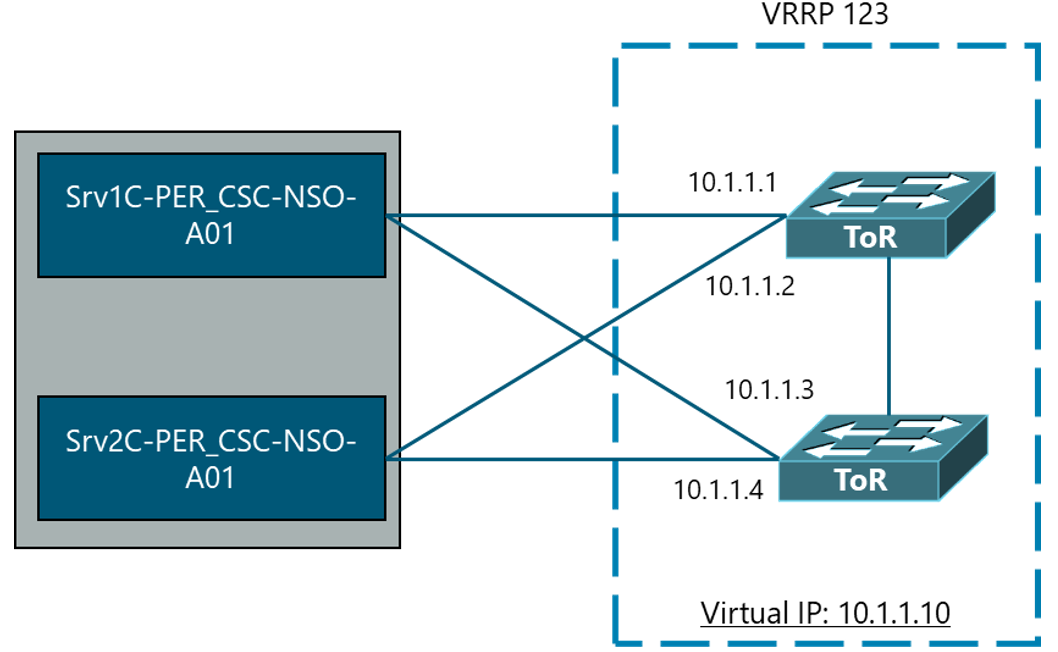
Figure 6. VRRP implementation for the vEPC servers with the ToR
Design Example
Routing and Switching Configuration:
The VLAN assignation would be as follows:
|
Interface |
VLAN Group |
|
O&M |
10 |
|
SGi |
100 |
|
Gx |
110 |
|
S8 |
120 |
|
S1-MME |
130 |
|
S1-U |
140 |
For communication to the equipment from partner MNOs, it is decided that for external Gx and S8, the use of BGP will be configured at the NFV solution and in the switch. For SGi, it will be implemented as a static route.
For S1-MME and S1-U there will be implemented through OSPF:
|
Interface |
Protocol |
Group ID |
Member Interfaces |
Networks/Subnetworks |
|
SGi |
Static |
NA |
Srv2C-PER_CSC-NSO-A01 (Port 0/5) Srv2C-PER_CSC-NSO-A01 Srv2C-PER_CSC-NSO-A01 (Port 0/7) Srv2C-PER_CSC-NSO-A01 (Port 0/8) SW1_ToR-PER_CSC-NSO-A01 (Port 1/7) SW1_ToR-PER_CSC-NSO-A01 (Port 1/8) SW1_ToR-PER_CSC-NSO-A01 (Port 1/9) SW1_ToR-PER_CSC-NSO-A01 (Port 1/10) |
Only the default route will be configured. 0.0.0.0/0 to the internet connected interface. IP subnets for all the port connections. |
|
Gx |
BGP |
100
|
IP address(es) for Gx IP subnets for all the port connections. |
|
|
S8 |
BGP |
110 |
IP address(es) for S8 IP subnets for all the port connections. |
|
|
S1-MME |
OSPF |
20 |
Srv1C-PER_CSC-NSO-A01 (Port 0/1) Srv1C-PER_CSC-NSO-A01 (Port 0/2) Srv1C-PER_CSC-NSO-A01 (Port 0/3) Srv1C-PER_CSC-NSO-A01 (Port 0/4) SW1_ToR-PER_CSC-NSO-A01 (Port 1/1) SW1_ToR-PER_CSC-NSO-A01 (Port 1/2) SW1_ToR-PER_CSC-NSO-A01 (Port 1/3) SW1_ToR-PER_CSC-NSO-A01 (Port 1/4) |
IP address(es) for S1-MME IP subnets for all the port connections. |
|
S1-U |
OSPF |
30
|
Srv2C-PER_CSC-NSO-A01 Port 0/1 Srv2C-PER_CSC-NSO-A01 Port 0/2 Srv2C-PER_CSC-NSO-A01 Port 0/3 Srv2C-PER_CSC-NSO-A01 Port 0/4 SW1_ToR-PER_CSC-NSO-A01 (Port 0/1) SW1_ToR-PER_CSC-NSO-A01 (Port 0/2) SW1_ToR-PER_CSC-NSO-A01 (Port 0/3) SW1_ToR-PER_CSC-NSO-A01 (Port 0/4) |
IP address(es) for S1-U IP subnets for all the port connections. |
It is important to note that this configuration must be implemented at the NFVI and Switch elements from the operators network plus the configuration on the partner MNO that should be consistent.
4.2.6 Interconnection Configuration
As the Diameter and GTP are the base protocols for the intercommunications between nodes within the EPC and to other operators cores, the interconnection configuration is needed for every EPC implementation. The main dependence is with R&S process since this enables the base communication for GTP and Diameter.
The first step of the interconnection is the identification of the needed configuration for the GTP interfaces. For inter EPC elements and to external networks.
The second step is the definition of the NAPTR DNS records according to section 3.3.1. It is important to remark that although these records are desirable to be in a DNS Server, they can be configured on the EPC equipment if the interconnection to MNOs is less than two.
As a third step, is the identification of diameter interfaces that need to be interconnected, their hostnames, IP addresses, transport protocol and port number accordingly to section 3.3.2.
Design Example
Interconnection Configuration:
Operator Data:
– MNC: 33
– MCC: 610
– CC: 86
For S8 interface (GTP-based), the first step is the GTP service bonding to the logical IP:
Bound [GTPv1 & GTPv2] to [10.96.0.69].
As a second step, it is needed a NAPTR DNS Record:
topoff.s8.pgw.node.epc.mnc33.mcc610.3gppnetwork.org (For further details on how to define the NAPTR record, see section 3.3.1)
For Gx interface (Diameter-based), it is needed some data for the protocol itself:
Hostname: Gx.pgw.NaaSOperator
IP Address: 10.101.0.X
Port Number: 3868
Work Mode: Initialize & Listen
Transport Protocol: SCTP
Supported Application IDs: 16777238 (Gx) [3GPP TS 29.212]
It is mandatory to configure the partner(s) diameter information if the Gx Interface is in Initialize work mode.
Partner Operator Data (Roaming): <-Previously gathered from partner MNO
– Hostname: Gx.pcrf.PartnerMNO
– IP Address: 200.1.0.201
– Port Number: 3868
– Work Mode: Listen
– Transport Protocol: SCTP
– Supported Application IDs: 16777238 (Gx)
4.2.7 Network Management Interfaces Configuration
Network Management Interfaces Configuration process is only needed when Operations / Business Support Systems (OSS/BSS) are planned to be implemented in the network for centralized management. As this step relies on proper communication between the OSS/BSS and the O&M interface of every equipment, it is highly dependent on the Routing and Switching Process.
The first step for this process is to define a VLAN for overall O&M and a Routing Protocol across the network, as detailed in section 3.2.
The second step would be to add all the network elements into the OSS/BSS systems for which, in some cases, it will be necessary to add them manually. In this case, the O&M IP for every NE needs to be included.
Design Example
Network Management Interfaces Configuration:
Step 1. The VLAN for O&M would be VLAN10 and the routing protocol would be OSPF with Group ID: 10, the network members would be all the O&M IPs, depending on the equipment which resides. The OSS/BSS System should be in the same VLAN10 to be able to communicate with all the O&M Interfaces.
Step 2. Add the O&M IP addresses manually into the OSS/BSS system.
4.2.8 EPC Network Element Configuration
As the EPC Network Element Configuration completely depends on the type of solution that is planned to be implemented, the minimum configuration will change from one to another. Table 12 contains the most common requirements for each NE and the ones which are common to all.
|
Description |
|
|
Common to all. |
IP information for all their interfaces (Service, O&M and Sync). |
|
GTP or Diameter Service Initialization (if not by default). |
|
|
Operator Information: Mobile Network Code (MNC), Mobile Country Code (MCC), Country Code (CC). |
|
|
MME |
Equipment Information: MME Group ID, MME Code, Date & Time. |
|
Interworking with eNB: Tracking Area Code (TAC), Location Area Code (LAC) & Routing Area Code (RAC) |
|
|
SGW Selection Policies (see section 3.3.2) |
|
|
SGW/PGW |
PGW/SGW Selection Policies (see section 3.3.2) |
|
Access Point Name (APN) Information (Charging Method (If any)) |
|
|
HSS |
Default User Profile, default APN, default Aggregated Maximum Bit Rate (AMBR), default QoS |
|
PCRF |
Default User Profile |
|
OCS/OFCS |
Default User Profile Parameters for measure user session/duration |
Table 12 Minimum Configuration Parameters for the EPC Network Elements
It is important to note that the policies which reside in the PCRF and the actions to be taken by the network will be defined in the following section.
Design Example
EPC Network Element Configuration:
For the MME the steps are:
– Configure its IP O&M, S11, S1-MME and S6a IPs. (Already defined in the IP allocation)
– Initialize the GTP Service and bond to proper interfaces
– Introduce MNC=33; MCC=610 and CC=86
– MME Group ID= 3000; MME Code=1
– Date and Time: server 0.north-america.pool.ntp.org
For the SGW/PGW the steps are:
– Configure its IP O&M, S11, S5/S8, S1-U, Gx and SGi IPs. (Already defined in the IP allocation)
– Initialize the GTP and Diameter Services and bond to proper interfaces
– Introduce MNC=33; MCC=610 and CC=86
– Date and Time: server 0.north-america.pool.ntp.org
– Default APN: internet.NaaS.com
For the HSS the steps are:
– Configure its IP O&M, S6a IPs. (Already defined in the IP allocation)
– Initialize the Diameter Service and bond to proper interfaces
– Introduce MNC=33; MCC=610 and CC=86
– Date and Time: server 0.north-america.pool.ntp.org
– User Default Profile: Data Service, 50000 kbps AMBR, Best Effort QoS (QCI9), using default APN
For the PCRF the steps are:
– Configure its IP O&M, Gx IPs. (Already defined in the IP allocation)
– Initialize the Diameter Service
– Introduce MNC=33; MCC=610 and CC=86
– Date and Time: server 0.north-america.pool.ntp.org
– User Default Profile: Policy & Charging Rules Configuration
4.2.9 Policy & Charging Rules Configuration
The Policy and Charging Rules Configuration is a process that can be avoided when no PCRF is present in the network and/or no charging/service differentiation is going to be considered in the design.
The main dependency is from the Logical and Physical Topology process and the service model already defined by the Operator.
The logic for the ruling establishment is done by selecting the criteria from Table 7 according to the subscription plans to be offered. Then, assign values for the threshold of every criteria and a set of actions to be performed by the network. These rules must be defined for every selected criterion and every one of them may contain one or more actions/thresholds.
Design Example
Policy and Charging Rules Configuration:
The plans for charging are desirable to be 0.5, 1 and 2 GB data consumption. And Apply a Bit Rate Modification from 10 Mbps to 386 kbps after the consumption threshold together with a different charging rate (From free to 0.1 USD per MB).
Change of QoS to QCI7 for VoIP to have a good quality during the calls.
There will be no restrictions for location nor roaming. And since there is no VoLTE service in the network, no profile for it is necessary.
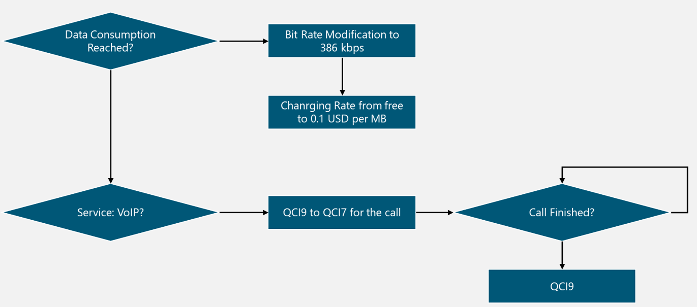
|
Criteria |
Threshold |
Action(s) |
|
Data Usage Consumption |
0.5, 1 or 2 [GB] |
Bit Rate Degradation 10 Mbps -> 386 kbps |
|
Charging Rate Modification Free -> 0.1 USD per MB |
||
|
Specific Service |
VoIP (Only during call duration) |
QoS/QCI Modification QCI9 to QCI7 |
Note: For allowing the VoIP service to modify the QoS, it is necessary that the NaaS Operator offers its own voice app. This way, the Mobile Core knows how to react to this specific application and avoid any vulnerabilities for third-party apps to modify the QoS at pleasure. This is also discussed on the Mobile Core Architecture Module.
4.2.10 Bill of Materials Generation
The Bill of Materials process is needed for every EPC implementation as this is the main input for the Purchase Order. The dependency for this BoM includes Equipment Selection and Dimensioning, Physical and Logical Topology and Interconnection Configuration.
The Equipment Selection and Dimensioning will indicate the equipment which would be handling all the traffic and it will be included in the BoM Generation.
All the connections included in the physical and logical diagrams indicate all the NICs, cables, optical fiber.
Finally, the interconnection configuration will indicate the number of connections to external networks thus complementing the NICs, cables, etc.
For all the aforementioned equipment, it must be specified the most relevant characteristics to avoid ambiguities.
The BoM Template can be used in order to ease the design, although the NaaS Operator can modify it to generate its own format.
Design Example
Bill of Materials Generation:
The summary of the material for the proposed solution:
|
Quantity |
Model |
Brief Description |
Price per Unit |
|
1 |
Vendor C Rack |
42 Unit Rack with dimensions: 2000x600x800 mm |
5,000 USD |
|
4 |
Vendor C NFVI vEPC |
Infrastructure from VendorB, 60 vCPU, 200GB RAM Memory & 500 GB Total Storage. |
25,000 USD |
|
2 |
Vendor B VNF Bundle |
vEPC VNF Bundle: MME, HSS, SGW & PGW. 480k SAU, 800k supported subscribers 12 Gbps data forwarding capacity. |
20,000 USD |
|
2 |
Switch from Vendor C |
1 Rack Unit Switch, 48 x 10GE + 4 1GE ports |
8,000 USD |
|
72 |
SFP+ Module |
Enhanced Small Form-factor Pluggable Transceiver, 10GE, SFF-8472 Compliant, LC-LC, FO, 850nm, 300m |
200 USD |
|
36 |
Fiber Optic Patch Cord |
LC to LC APC Duplex OS2 2.0mm PVC Fiber Patch Cable, 10m |
100 USD |
5 LLD Recommendation
Methodology to consolidate and generate a final LLD recommendation.
5.1 LLD Recommendation Format & Structure
The main deliverable is the LLD recommendation, which contains the overall technical solution, design rules, the most common parameters per protocol in the Mobile Core Network. The LLD recommendation shall contain the following aspects:
5.2 LLD & BoM Recommendation Generation
Generation of the LLD Recommendation following the format and structure established. NaaS Operators can use the LLD Report Template and the BoM Template as a reference to create their own version.
1. Civil Power CORE Introduction
Civil and Power Design for Core Sites refers to the process performed to assess and dimension the Power Equipment to properly energize the equipment at Core Sites and design the arrangement of the whole system considering as inputs the assigned space diagrams, Core LLD and Core Equipment engineering requirements, to design a proper Power Solution and a Core Site Layout. An accurate Power and Civil design will achieve economically efficient Power Feed Solution providing more availability and reliability.
In contrast to Civil & Power Design for RAN Sites, Core Sites have a much higher energy consumption and ideally, their availability should be close to 100% per year. In addition, Mobile Core facilities differ in size and type, from NaaS Operator-owned facilities, to 3rd party aggregation nodes or data centers.
The Civil and Power for Core Sites Module provides the NaaS Operator with background information to aid in the selection and design of a customized Power System for their Mobile Core Equipment and guides NaaS Operators to prepare their Core Site Layouts that will define the position of all Core & Power components in blueprints.
The Core Power Design assesses the Power Feed Options that suit the Core scenario which can be AC or DC. When the Power Feed option has been established, the next step is to match the selected Core components requirements and Autonomy requirements with power systems capabilities, optimizing cost and protecting the NaaS Operator Hardware Investment. Once the Power Hardware is established NaaS Operators will be able to generate the Power Equipment Bill of quantities for Core Sites and the Core Site Layout must be performed, indicating where the hardware must be installed, facilitating the forthcoming Installation & Maintenance Task.
1.1 Module Objectives
This module will guide NaaS Operators to accurately assess and dimension the Power Equipment for the Core Sites and develop the Core Site Layouts that will define the equipment location, ensuring their right installation and operation. The specific objectives of this module are to:
1.2 Module Framework
NaaS Runbooks Framework shown in Figure 1 displays the Runbook modules and their relationship to the Civil & Power Design for Core Module.
The Civil & Power Design for Core Module is included within the Network Design Stream. It takes inputs from the Core LLD Module and the output generated serves as guidelines for equipment installation at core sites in the Deployment stream.
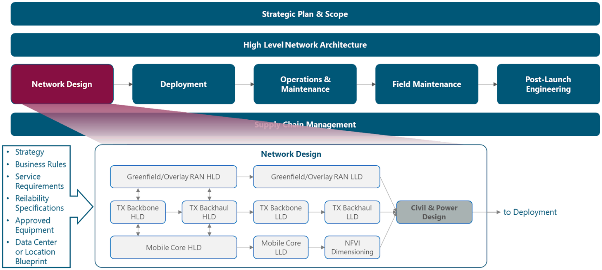
Figure 1. Runbook Framework.
Figure 2 presents the Civil & Power Design functional view where the main functional content of the module is exhibited.
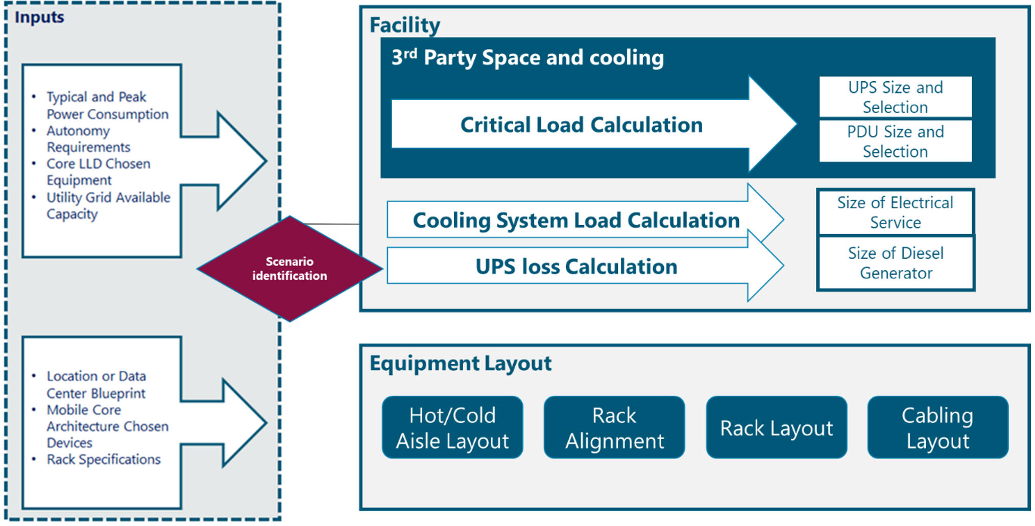
Figure 2. Civil & Power Design Functional View.
The rest of the module is divided into three sections. Section 2 is an introductory section, containing a high-level view of the Civil & Power Design for Core Sites, their main characteristics, and functions. Section 3 contains the key considerations used to design a power solution that properly fits the requirements of the core equipment, Section 4 is a set of guidelines to organize and prepare the Core Site layout following NaaS Operators assigned space for the Mobile Core Equipment or Data Center physical Characteristics.
2 Civil & Power Design Fundamentals
The Core site refers to the facility and physical elements that support the mobile Core equipment. The Core site must be designed to meet the power and environmental requirements of the Core equipment with the maximum availability of noise-free electrical power avoiding single point of failure circumstances. This section introduces the basic knowledge before getting into the details to perform a Power system Design for NaaS Operator Core sites.
2.1 Civil & Power Design Overview
Core site power systems require in-depth evaluation at the design stage, in order to balance the need for maximum system availability and an economically feasible power solution that suits the chosen equipment at the Low-Level Design Stage. As established in the Mobile Core Architecture Module, the recommended option for NaaS Operators is to implement the Mobile Core through Network Functions Virtualization (NFV), which virtualizes the functions of the Evolved Packet Core (EPC) in traditional IT equipment. This makes it possible to use traditional power systems used in the IT industry which are mainly for alternating current (AC).
Once the Power and Core equipment has been decided, the equipments layout must be defined which can be within the equipment room or data center facility.
The importance of a properly designed power system is explained in the following statements:
2.2 Civil & Power Design Scenarios
The Core Site Design requirements directly depends on the scenario in which the core equipment will be deployed. The scenario is normally decided in previous phases according to the NaaS Operator strategy. The variety of scenarios can fall into the following categories:
The required tasks for each scenario are shown in Figure 3 and described below:
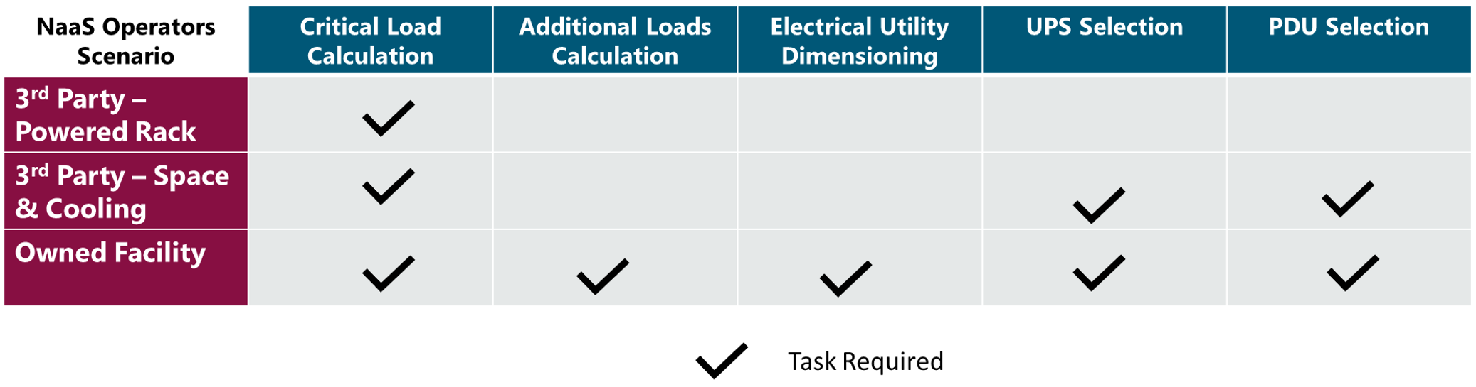
Figure 3 Mobile Core Deployment Scenarios and related Power Design tasks.
Each of these tasks is described with a deep detail in Section 3.
2.3 Civil & Power Design Inputs Description
To perform an optimized design, a set of inputs from various sources is required. This section identifies the most important inputs and how these inputs impact the Civil and Power Design for Core Sites.
Table 1 lists the inputs for Civil & Power Design, showing the impact on the overall process and potential sources.
|
Input Required |
Description |
Impact |
Source |
|
Equipment Power consumption (W), Average Load |
Power Consumption of the Core system. |
Required to properly Size the Power and Electric System Elements |
Mobile Core LLD Vendor Specifications, Vendor sizing tools |
|
Power Equipment Specifications |
Specifications of all Power Equipment: Power INPUT: ● Voltage Range ● Frequency ● Maximum Current Power OUTPUT: ● Voltage Range ● Maximum Power ● Maximum Current ● Peak Efficiency |
Required to properly size and select the Power System Elements |
Vendor Specifications |
|
Site Engineering |
Contains detailed blueprints corresponding to each site. |
Required to define the Site Layout |
Site Construction Module / Contractors |
Table 1 Civil & Power Design Inputs
2.4 Power System Overview
A core power system is the electric network within the core site which consists of distribution and transformation of the electricity from the public electric network or so-called Grid. The electricity from the Grid must be reduced to lower voltage levels using a transformer and then is distributed before it can be delivered to the Core equipment.
In North America, parts of Central and South America, Japan, and Saudi Arabia, the electricity is distributed using transformer-based Power Distribution Units (PDUs) which are typically 480 VAC. The transformer steps down the voltage, and power is delivered to the equipment at 208/120 VAC. For the rest of the world, the power distribution uses 400/230 VAC or 415/240 VAC.
A power supply unit (PSU) embedded in the equipment, step down the voltage to 12VDC and lower DC voltages for internal uses.
DC power in data centers is being used as an alternative to AC. In this model, AC power is delivered to the rack and is converted to DC prior to the distribution of power within the rack. However, this approach places some undesirable constraints on the deployment options when compared with traditional AC power distribution, which has prevented its wider adoption. Due to this constrains this module will be based on the most common distribution which is the AC Power.
The Power Design complexity depends on the size of the power load demanded by the IT equipment.
When NaaS Operators just need to feed a few servers, storage, and IT equipment pre-assembled power systems are the most adequate option.
Figure 4 shows a Power System to power up a small virtualized EPC, including the basic elements of the Power System: Power distribution system, Cooling system, Uninterruptible Power Supply (UPS), battery pack, and IT equipment space integrated into a standard 42U rack.
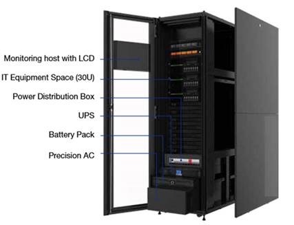
Figure 4. Rack for 30U backed by a single UPS
In cases where the vEPC requires a higher power demand or several racks, NaaS Operators may consider to assemble their power distribution system to feed their equipment. There are multiple Power system solutions available that NaaS Operators may consider, the criteria for choosing a solution will depend on several factors that will be deeply evaluated in Section 3.
Typically, the amount of electrical load and required availability its the key factor to consider in a power distribution system. There are many different loads in the Core Site, such as IT equipment, air conditioners, fans, lights, etc. The flow and transformation of energy from the utility/generator to the load is enabled by various types of equipment:
As described in Section 2.2 depending on the scenario, not all the electric and power equipment is the responsibility of the NaaS Operator: depending on their scenario NaaS Operators may just require to ensure that their core equipment is properly fed in a 3rd party facility or they may have to design the power system for the whole facility including the power distribution system. This is illustrated in Figure 5, which shows all the elements of a basic Power System.
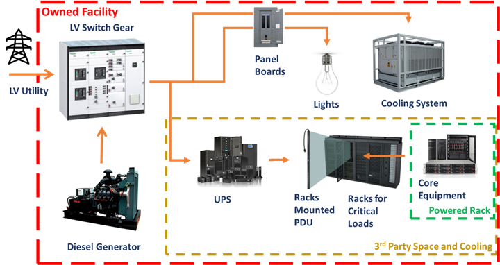
Figure 5 Full Sized Power System for a Core Site.
The following subsections introduce each type of equipment.
Typically, LV switchgear/switchboard is located in the electrical room and marks the utility service entrance for facilities with a power load of less than 1 MW.
If a Diesel generator is used, the generator would feed the LV switchgear. Apart from distributing power, the LV switchgear is responsible for disconnecting faults and controlling the LV power distribution system. A device known as an automatic transfer switch (ATS) has traditionally been used to switch between utility and generator. However, the current trend is to have LV breakers perform this function in lieu of the ATS device. If the NaaS Operator considers purchasing a Low Voltage Switchgear and a Diesel Generator, it is recommended to look for electrical consultants services to size and select the Switchgear.
Panelboards (typically rated from 1.5kVA to 75kVA) are basically a metal cabinet that houses the main electrical bussing and the terminals upon which circuit breakers, neutral wires, and ground wires are installed. Panelboards are common in the mechanical space, electrical space, and IT space to distribute the power to cooling equipment (i.e. chillers, pumps, fans, etc.), lighting, and security devices.
UPSs are typically installed to provide uninterrupted power to the critical equipment. This piece of equipment is in charge of distributing quality electricity by conditioning the AC power to ensure that electrical issues like power surges do not impact the equipment.
In addition to power conditioning, UPS systems are used to store electricity in batteries. UPS provides backup power when utility power fails, either long enough for critical equipment to shut down gracefully so that no data is lost, or long enough to keep required loads operational until a generator comes online, which is commonly 10 or 20 minutes. If a Generator is not included in the system design NaaS Operators may consider extending the emergency power supply of the UPS with additional batteries; however, not all UPS support a battery extension.
The chosen UPS directly impacts the availability of critical Core equipment. The Methods to properly select the UPS are addressed in Section 3.3.
PDUs are used to distribute, control, and monitor the critical power from the UPS system to equipment racks. PDUs usually contain a main input circuit breaker, branch circuit panelboard(s), a power transformer, output power cables, surge arrestor, and the monitoring and communication modules.
Sometimes PDUs with power transformers are used to decrease voltage levels; for example, in North American data centers, PDUs with power transformers are mainly used to step down 480 Vac to 120/208 Vac8; while in Japan, PDUs with power transformers step down 200Vac to 100Vac single-phase for the downstream IT loads. A PDU is typically rated from 50kW to 500kW.
For low power critical loads rack PDUs are used instead of Factory-configured PDU distribution systems within dedicated enclosures or cabinets. Rack PDUs (i.e. power strips) are installed on the equipments rack and are powered from the UPS connector. Rack PDUs distribute power directly to equipment in the rack. PDUs are selected based on the expected rack power density and or system configuration. The method to properly select a PDU is addressed in Section 3.4.
It is a common practice to use diesel generators to supply power to the data center or core facility in case of an outage from the main grid power source, delivering energy as alternating current (AC). Backup diesel generators serve to keep the facility operational for a longer period of time. The length of time is dependent on the amount of onsite diesel fuel storage and the delivery of fuel which is referred to as fuel contracts. This can be hours, days, or weeks. The method to calculate the required capacity of a diesel generator is detailed in Section 3.6.
2.5 Core Site Layout Overview
The Site Layout for Core Sites refers to the technical drawings that show information about power and core site equipment. The Site Layouts are created and used by engineers, builders and field technicians; they consist of lines, special symbols, dimensions, and notations. The Site Layout shows the scheme of electric wiring and position of power and IT equipment in buildings, or data centers.
As explained before, two types of locations for Core Sites are commonly used by NaaS Operators:
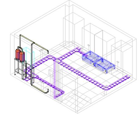
Figure 6. NaaS Operator Core site layout
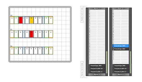
Figure 7 Shared Data Center Layout for NaaS operators Core equipment
3 Power System Design
This section provides guidelines for collecting and preparing the necessary information and the procedures to dimension and select the basic components of the power distribution system that feeds a Core site.
3.1 Power System Design Process
To ensure the Core Site always ends up with the right power system, NaaS Operators may consider the following process:
Firstly, NaaS operators should identify their scenario as was described in Section 2, then the load calculation of the equipment is performed in order to properly size and select the UPS system and PDU. If NaaS operators decide to build their own facility the electrical distribution design must be performed, and the additional loads such as cooling and lights must be calculated in order to calculate the overall capacity of their facility and optionally size a diesel generator and switchgear. This process is represented in the diagram of Figure 8.
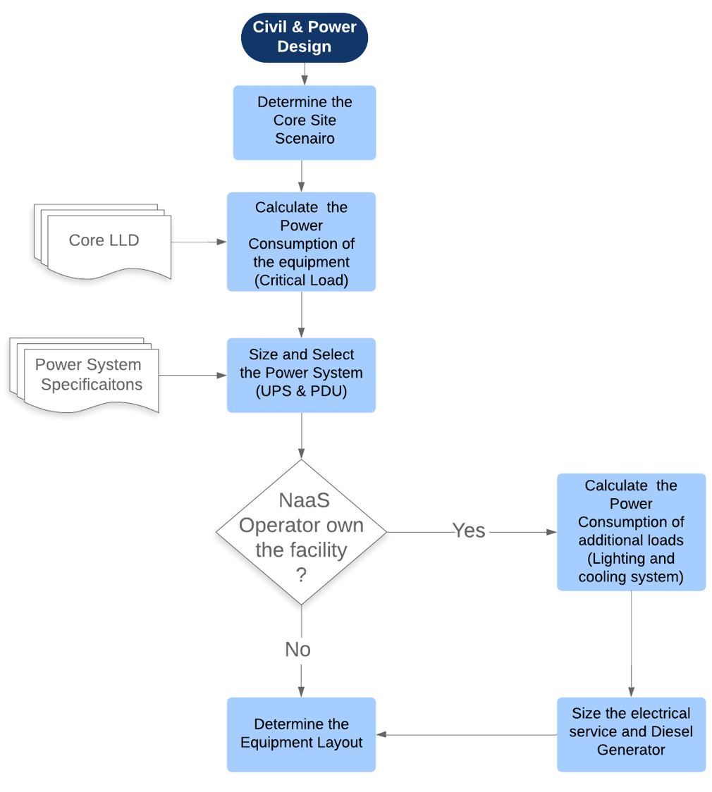
Figure 8 Civil and Power Design for Core Sites Process Diagram
The following sections will provide methodologies to assist NaaS Operators in each step of the Power System Design.
3.2 Critical Load Calculation
The critical load is all of the hardware components that make up the NaaS Operators Core site: servers, routers, storage devices, telecommunications equipment, etc. The Critical Load Calculation is used to choose the right UPS that will protect the equipment and guarantee a certain level of availability. If the Design will be performed at the facility level the critical loads include security systems, fire and monitoring systems that protect the equipment. The following steps will assist in estimating the capacity required for the critical load:
3.3 UPS Sizing and selection
In order to size and select a UPS that protects the Critical Loads in an efficient way, this section provides guidelines to properly choose a UPS based on the UPS design options, the required capacity or rate that the UPS must provide and UPS form factor options.
3.3.1 UPS Design Options
A variety of design approaches are used to implement UPS systems, each with distinct performance characteristics. The most common designs used in core facilities and data centers are:
The following subsections provide a short description and recommendations to choose between these different designs.
3.3.1.1 The line-interactive UPS
The line-interactive UPS, illustrated in Figure 9, is the most common design used for small data centers. In this design, the battery-to-AC power converter (inverter) is always connected to the output of the UPS. In this way, the inverter operates in reverse mode when the input AC power is normal providing battery charging.
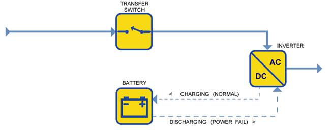
Figure 9. Line-interactive UPS
When the input power fails, the transfer switch opens and the power flows from the battery to the UPS output. With the inverter always on and connected to the output, this design provides additional filtering and yields reduced switching transients when compared with the standby UPS topology.
In addition, the line-interactive design usually incorporates a tap-changing transformer. This adds voltage regulation by adjusting transformer taps as the input voltage varies. Voltage regulation is an important feature when low voltage conditions exist, otherwise, the UPS would transfer to the battery and then eventually down the load.
For NaaS Operators whose critical load is in the 0.5 to 5 kVA power range, the recommended option is the line interactive design due to the High efficiency, small size, low cost and high reliability coupled with the ability to correct low or high line voltage.
3.3.1.2 The double-conversion online UPS
In the double conversion on-line design, failure of the input AC does not cause activation of the transfer switch, because the input AC is charging the backup battery source which provides power to the output inverter. Therefore, during an input AC power failure, on-line operation results in no transfer time. Both the battery charger and the inverter convert the entire load power flow in this design.
This UPS provides nearly ideal electrical output performance. But the constant wear on the power components reduces reliability over other designs. Also, the input power drawn by the large battery charger may be non-linear which can interfere with building power wiring or cause problems with standby generators. The block diagram of the double-conversion on-line UPS is illustrated in Figure 10.
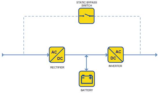
Figure 10. Double conversion online UPS
Generally, double-conversion online UPS provides higher availability. Using the static bypass switch allows maintenance of the system without interrupting the power supply. Additionally, this provides the highest levels of protection, completely isolating the critical load from the utility during normal operations.
Double conversion online UPS is highly recommended for critical loads that demand more than 5KVA.
3.3.1.3 The delta conversion on-line UPS
This UPS design, illustrated in Figure 11, eliminates the drawbacks of the double conversion on-line design and is available in sizes ranging from 5 kVA to 1.6 MW. Similar to the double conversion on-line design, the delta conversion on-line UPS always has the inverter supplying the load voltage. Under conditions of AC failure or disturbances, this design exhibits behavior identical to the double conversion on-line. However, the additional delta converter also contributes power to the inverter output which the most important benefit is a significant reduction in energy losses.
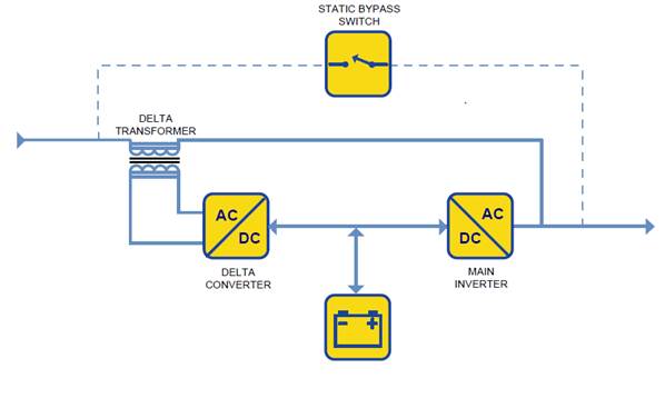
Figure 11 Delta conversion online UPS
However, Delta conversions online UPS have a higher cost per VA compared with other designs. Which made a Delta conversion online UPS a good option for critical loads that demands more than 10 kVA.
Table 2 shows some of the characteristics of the various UPS types. Some attributes of a UPS, like efficiency, are dictated by the choice of UPS type:
| |
Practical power range (kVA) |
Voltage Conditioning |
Cost per VA |
Efficiency |
Inverter always operating |
|
Line interactive |
0.5-5 |
Design Dependent |
Medium |
Very High |
Design Dependent |
|
Double conversion on-line |
5-5000 |
High |
Medium |
Low-Medium |
Yes |
|
Delta Conversion on-line |
5-5000 |
High |
Medium-High |
Medium |
Yes |
Table 2. UPS characteristics
3.3.2 UPS Capacity Ratings
The watt rating of the UPS relates to the amount of power it can deliver, and the VA rating of the UPS relates to the amount of current it can deliver. Neither the Watt nor the VA rating of the UPS can be exceeded.
In practice, the best approach to size a UPS is to use the Watt rating of the load. If there is confusion regarding power ratings, and it is desirable to ensure the load can be powered by the UPS, then choosing a UPS with a Watt rating greater than or equal to the VA rating of the load will always ensure a safety margin. Additionally, the UPS efficiency should be considered.
UPS efficiency is based on how much of the original incoming power is needed to operate the UPS. For example, an uninterruptible power supply with a 95% efficiency rating will have 95% of the original input powering the load and connected systems, with the remaining 5% energy wasted running the UPS.
For a UPS, higher efficiency equates to lower losses of electrical energy in terms of heat output low-efficiency UPS often require more air conditioning to help keep ambient temperatures safe.
Even a 1% or 2% improvement in operating efficiency can add to up substantial energy costs over the full-service life of a UPS (i.e. approximately 10 years), particularly for larger systems with higher power ratings. However, in any discussion about UPS efficiency, its worth keeping two things in mind:
The efficiency ratings that UPS manufacturers publish are based on running in online operating mode with a 100% fully rated load. But as the load reduces, so does UPS efficiency. As an example, a UPS running at 20-25% load may only be capable of 85% efficiency. In practical terms, a realistic and sufficiently accurate value for UPS efficiency for a typical installation is 88%. This approach is summarized in Equation 1:
![]()
(Eq. 1)
This method is illustrated in the following example:
Example:
Estimate the UPS rate if the critical load connected to the UPS consume 1200W.
Solution:
Using Eq1:
![]()
Therefore, the required UPS must be capable to provide at least 1365W
3.3.3 UPS Form Factor
UPSs come in a range of form factors that fit into two master categories: rack-mounted and freestanding. High rated UPSs are not available in rack-mounted form factors, so companies with substantial power requirements almost always use freestanding devices.
For NaaS operators with more modest needs, deciding between rack-mounted and freestanding UPSs is largely a matter of design preference. Some organizations use rack-mounted UPSs in an effort to consolidate as much hardware as possible in their enclosures. Others prefer to maximize the amount of rack space available for servers by using freestanding UPSs.
From a technical and financial standpoint, neither approach is inherently superior to the other. Figure 12 shows different form factors for UPS ranges from 700 VA to 1100 kVA.
A use case example of the Rack Mount is in the scenario where NaaS Operators lease a space within a data center. In this case, the available space becomes a priority to consider.
Commonly, Rack Mount UPSs are used for low power consumption configurations of less than 20kVA and are installed close to the critical loads. The high rated UPS of more than 20kVA is used in Centralized configurations. The high rated UPS is designed to be a central backup for multiple loads.
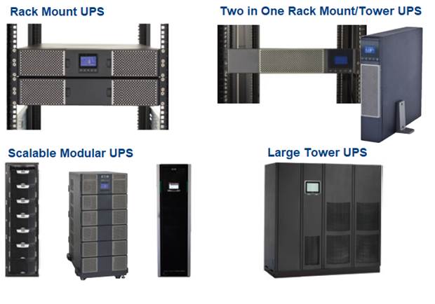
Figure 12. UPS Form Factors
NaaS Operator may consider rack mount UPS if is not planed a growth of the required IT equipment within the rack. However, if it is planned to add more equipment, NaaS Operators may consider Scalable Modular UPS to allow more space within the rack and add more power capacity if it is required.
In cases where the Critical load exceeds 20kW NaaS Operators should consider a Large Tower UPS as a centralized unit. In this case is suggested that NaaS Operators look for electrical consultant services to properly design the architecture and select the right equipment for their core site.
3.3.4 UPS Evaluation Matrix
After selecting the UPS type, capacity and form factor, there are additional considerations to select a UPS. A best practice is to narrow down to a few different UPS models, NaaS Operators may use Table 3 as a checklist to evaluate competing vendors.
|
Factor |
UPS 1 |
UPS 2 |
|
Voltage Be sure the input and output voltages are the same. |
|
|
|
Input plug Do both UPSs have the same input plug? Does it match the wall socket? UPSs 1500 VA and below can be plugged right into a standard wall socket. Larger models may require an electrician to install a new wall socket. |
|
|
|
Output receptacles Does each UPS have the same quantity of output receptacles? The same type? Be sure the UPS has enough output receptacles and that theyll accommodate the power cords of the servers, etc. |
|
|
|
Warranty Are the warranties the same duration? How long does the warranty cover the batteries? |
|
|
|
User interface Do both UPSs utilize the same interface? Do both have an intuitive LCD or basic LEDs? |
|
|
|
Network card Is remote monitoring required? Does the UPS include Network card? Some UPSs include a card while others dont, and this can impact the price. In cases where the Core site accessibility is not granted is a good option to consider a UPS with a Network card. |
|
|
|
Software Do both UPSs have equivalent software capabilities? For example, if integration into VMware vCenter is a priority, be sure the UPS software can do it. |
|
|
|
Mounting hardware The UPS will be mounted in a rack enclosure or 2-post rack? If the mounting is not included with the UPS, will be required to purchase the hardware separately. |
|
|
|
Rack height If a rack mount UPS is selected, are they of the same rack height (U)? For example, going with a 1U UPS over a 2U model may allow to fit another server in the rack. |
|
|
|
Maintenance bypass It has been considered the price of a maintenance bypass module that will allow to keep the IT equipment up and running if it is needed to replace the UPS or if the UPS fails? |
|
|
|
Batteries It has been considered the cost of additional battery packs? The cost of replacing the batteries in the UPS? |
|
|
Table 3. UPS Evaluation Matrix
3.4 Power Distribution Unit Selection
Power distribution units (PDU) are available with a variety of different features, power ratings, and input and output cord combinations. Depending on the architecture, PDUs may act as a centralized unit to distribute the power to a row of racks or distribute the power directly to the IT equipment mounted inside the rack.
Centralized PDU may have several regulated outputs for multiple loads, typically this type of PDUs are rated from 50kVA to 500kVA. In this case, NaaS Operators may look for assistance with PDUs vendors, to select the PDU suited for large, centralized architectures.
This section provides guidance to select the rack PDU suited for small deployments for less than 50KVA.
- Determine output plug type and quantity
The first decisions are made based on the application inside the rack. IT equipment in racks can have several different plug types. The most common plug types in data centers are C-13 and C-19 connectors (see Figure 13). C-13 connectors are usually found on servers and small switches, while blades and larger networking equipment use the C-19 plug because of its higher current carrying capacity.
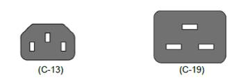
Figure 13 Output Plug Types
NaaS Operators must verify the plug type that each IT equipment requires and ensure that the PDU has enough output plugs for each type.
- Select form factor and mounting
Commonly, each piece of hardware has redundant power supplies intended to provide power in case the other fails. For data center applications, these power supplies are generally connected to separate redundant rack PDUs which are, in turn, fed from separate sources or circuits. This prevents the entire load from dropping in the event of a fault along one power path.
Rack PDUs install into the back of a server cabinet and provide convenient outlets accessible to both IT equipment and users that must configure the equipment. Two primary mounting orientations, illustrated in Figure 14, are:
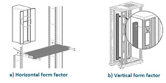
Figure 14 PDU Form factor
3.5 Total electrical capacity calculation
In case that NaaS operators decide to design their own power distribution system for their facility, the total electrical capacity should be calculated in order to size the electrical service form the Grid and optionally size a diesel generator.
Different power loads have been determined to estimate the size of the electrical system that will power the core facility or data center:
In general, the electrical supply must be large enough to support the sum of these loads. Underestimating the required capacity may result in future power disruptions, and overestimating leads to excessive initial installation costs and higher ongoing maintenance expenses.
3.5.1 UPS Loss Calculation
The total electrical capacity must include a factor for the inefficiency of the UPS system as well as the additional power required for battery charging. Following the practical approach described in Section 3.3.2 it is possible to assume the UPS efficiency at 88%. Please note that with high consumption applications the best approach is to contact UPS manufacturer to obtain the real efficiency of the UPS according to the connected load.
Battery charging is a significant but intermittent power consumer. Under normal operation with a charged battery, the charging load is negligible. However, when the battery load has been partially or completely discharged, the battery charging power can be on the order of 20% of the rated UPS load. Although this load is not likely to occur, the generator and service entrance must be sized considering this load.
This can be summarized in the following equation:
![]()
(Eq. 2)
Equation 1 is illustrated with the following example:
Example:
Calculate the UPS loss if the critical load connected to the UPS consume 1200W and the selected UPS have a rate of 2000W
Solution:
Using Eq1:
![]()
3.5.2 Cooling loads
Servers and related equipment generate a considerable amount of heat in a relatively small area, this is known as the heat output. The total heat output of a system is the sum of the heat outputs of the components. The complete system includes the Core equipment hardware, plus other items such as UPS, Power Distribution, Air Conditioning Units, Lighting, and People. Fortunately, the heat output rates of these items can be easily determined via simple and standardized rules:
- The power transmitted by core equipment through the data lines is negligible. Therefore, the power consumed from the AC power mains is essentially all converted to heat. This fact allows the use of the equipment power consumption in watts as the heat output.
- The heat output of UPS and Power Distribution systems consists of a fixed loss and a loss proportional to operating power, PDUs heat loss behave in a similar way. These losses are sufficiently consistent across equipment brands and models, so they can be approximated without significant error. The heat output of the UPS system is calculated using Equation 3 and the heat loss of a PDU using Equation 4
- Lighting and people can also be estimated using standard values. The only information needed to determine the heat output is the floor area in square meters, and the maximum number of people.
![]()
(Eq. 3)
![]()
(Eq. 4)
![]()
(Eq. 5)
![]()
(Eq. 6)
The total cooling loads is the sum of each heat load. NaaS Operators may use the Heat load calculator to determine the total heat output of a data center quickly and reliably.
The calculation of the heat load is illustrated in the following example:
Example:
Calculate the power load consumed by a cooling system in a room of 10 m2 that allows a max of 3 people. The Critical Load Power consumption is 1500W.
The Selected UPS have the following characteristics: 120V, 2kW, and includes a PDU.
Solution: From Equation 2, Equation 3,Equation 4, Equation 5
![]()
![]()
![]() = 215.3W
= 215.3W
![]()
Total:155W+50W+215.3W+300W=720.3W
3.5.3 Light Power Consumption
The lights power consumption follows the same approach as their heat load and is possible to use the same expression for their power calculation. As is indicated in Eq. 5.
3.5.4 Final electrical calculation
The steady-state power consumption of the loads within a data center establishes the power consumption for purposes of determining electrical costs. However, the electrical service and the generator power sources that provide power to the facility cannot be sized based on the steady-state values, but using the peak power consumption of the loads, plus any derating or oversizing margins required by code or standard engineering practice. The Total electrical capacity can be calculated using equation
![]()
(Eq. 7)
Figure 15 shows the Load distribution in a typical data center, considering the cooling system, lighting, UPS inefficiency and Critical Loads.
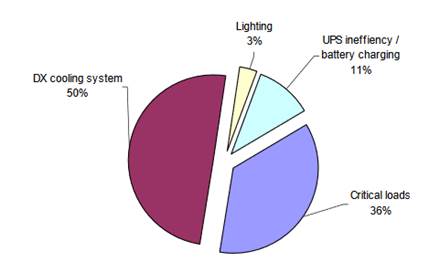
Figure 15. Load estimation for a data room used for Core equipment
Once the total electrical capacity is estimated in kW from Equation 6 two critical determinations are made: an estimate of the electrical service needed to supply the data room, and the size of any standby power generator capacity, if required.
The electrical service can be calculated as follows:
![]()
(Eq. 8)
Where :
![]() = Three-phased Utility Voltagep>
= Three-phased Utility Voltagep>
![]() = Formula Used for Three-phase utility
= Formula Used for Three-phase utility
![]() = Formula Used for Single-Phase utility
= Formula Used for Single-Phase utility
The utility volts are multiplied by 1.73 due to the phase relationship, neither voltage nor current flow applied to an IT load ever drops to zero. This means three-phase power at a given voltage can deliver more power. In fact, about 1.73 times the power of a single-phase supply.
This provides an estimate of the current capacity required to support the critical load, cooling, and building functions for a core facility. The following example illustrates the calculation of the required capacity.
Example: Calculate the electrical capacity of a core facility (data room) with the following load consumptions:
1.-Critical Load: 1200W
2.-UPS loss: 564W
3.-Lights: 216W
4.-Cooling System:720W
5.-Thre-phase voltage: 230V
Solution:
From Eq.7 :
![]()
![]() = 1500W + 564W + 216W + 720W = 3000W
= 1500W + 564W + 216W + 720W = 3000W
From Eq.8:
![]()
3.6 The use of a Generator in IT applications
While UPS systems today provide excellent protection from utility mains transients and short-term blackouts, they are not a complete solution for applications that must remain online 24/7, without interruption. A power outage that exceeds the UPS battery autonomy is always possible, yet a system shutdown, even if managed gracefully, is not acceptable. Running the application from additional UPS batteries is pointless if there is no power for the air conditioning system that cools the IT equipment and the batteries.
A standardized solution is to complement the UPS system with a backup generator that starts up if the battery autonomy is threatened, then runs indefinitely if necessary. The UPS bridges the power gap between the mains failing, and the standby generator starting up and reaching synchronization. It also cleans all power, whether from the mains or the generator.
The generator in a data center is used to reach the availability requirements. The availability of the data center refers to meeting the uptime expectations of the users. The Uptime Institute suggests a four-tier system, where each level describes the required availability. The higher the tier, the greater the availability.
The lowest cost and the lowest performance data center, Tier I, has a target availability of 99.671 percent, which translates to 28.8 hours of annual IT downtime. The highest-level data center design, Tier IV, has a target of 99.995 percent availability, or 24 minutes of annual IT downtime. In rural deployments, core sites are located in Tier I or Tier II. Table 4 shows an analysis of the Tier classification:
|
|
Tier I |
Tier II |
|
Utility Voltage |
230V, 480V |
230V, 480V |
|
Yearly IT downtime |
28.8 Hours |
22 Hours |
|
Site Availability |
99.671% |
99.749% |
|
Recommended for |
$13,500 – $18,000 / rack |
$18,000 – $24,000 / rack |
|
Historical Uses |
● Small businesses ● Data centers typically below 100 kW of IT capacity |
● Small to medium businesses ● Data centers typically below 500 kW of IT capacity |
|
Reasons for use |
● Reduce capital cost and energy cost ● Support for lower criticality applications ● Simple configuration and installation ● Ability to bring down load for maintenance |
● Improved fault tolerance ● Ability to use different UPS models ● Ability to increase future capacity |
Table 4 Datacenter availability classification
If NaaS Operators considers that Tier I exceed their characteristics, then the evaluation to purchase a generator can be made as follows:
If the Yearly Downtime from the grid will produce greater loss than the cost of a generator in a year, NaaS Operators may consider to purchase a generator. This is illustrated with the following formula:
![]()
(Eq. 9)
If the criteria established in equation 9 result false NaaS Operators may consider to purchase additional batteries for the UPS (if supported). Most of the UPS vendors offer to size the batteries for their UPS as part of their service.
The Tier I architecture is shown in Figure 16, please note that the availability indicated in Table 4 is achieved with the use of a Generator and a UPS together.
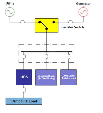
Figure 16 Tier I architecture
The following subsection contains guidelines to size a generator based on the loads of the Core site.
3.6.1 Sizing a Standby Power Generator
Once the size of the electrical service has been determined, consideration can be given to dimension a standby power generator, which will provide power in the event of a utility failure effectively improving the availability of the data center.
To estimate the size of the generator required for the total loads, use Equation 10, which considers the electrical characteristics of the loads to be attached to the generator through the transfer switch. Mechanical loads, like cooling loads, require high starting currents which are reflected by multiplying by 1.5 the cooling loads:
![]()
(Eq. 10)
The type of UPS will impact UPS-generator compatibility and configuration, as not all can compensate for frequency variations without relying on the battery. To ensure that optimal UPS vs generator sizing is achieved, it is recommended to consult with both the UPS and the generator manufacturer prior to finalizing a purchase.
4 Core Site Layout
Core Site Layout consists of the design considerations of the room and the layout of the Core equipment in the Room and the rack.
A Core site layout has two components: the structural layout of the empty room which may be obtained from the site engineering in the form of blueprints and the equipment layout of what will go in the room. Note that in the case where NaaS Operators decide to lease a space in a data center, the room is pre-existing, and the only option is to layout the equipment in their cabinet.
The equipment layout shows the footprint of IT equipment and the footprint of power and cooling equipment. In order to protect the IT equipment from overheating the layout should consider an airflow path. The following subsections provide guidelines to layout the rack in a room considering the airflow of the equipment, the equipment layout within the rack as well as key considerations for the cabling layout.
4.1 Control of airflow using hot-aisle/cold-aisle rack layout
The use of the hot-aisle/cold-aisle rack layout method is well known and commonly used in a data room layout. The basic principle is to maximize the separation between IT equipment exhaust air and intake air by establishing cold aisles where only equipment intakes are present and establishing hot aisles where only equipment hot exhaust air is present. The goal is to reduce the amount of hot exhaust air that is drawn into the equipment air intakes. The basic hot-aisle/cold-aisle concept is shown in Figure 17.
Figure 17. Basic hot-aisle/cold-aisle layout plan
In Figure 17, the rows represent the IT equipment enclosures (racks). The racks are arranged such that the adjacent rows face back to back, forming the hot aisles. The benefits of the hot-aisle/cold-aisle arrangement become dramatic as the power density increases. When compared to random arrangements or arrangements where racks are all lined up in the same direction, the hot-aisle/cold-aisle approach allows for a power density increase up to 100% or more, without hot spots, Decreasing greatly the power consumption of the cooling system.
4.2 Server Rack Layout
In terms of layout, rack density should be considered. The more free-space within a server rack, the greater the room for airflow. Vertical space can be left between servers and IT devices to help cooling. Heat sensitive devices, including UPS batteries, can be placed towards the bottom of a server rack. Heavier devices are also best placed towards the bottom of a rack.
Hardware should ideally be logically grouped for ease of management and access to sockets, outlets and ports, whether for power or networking. Ideally within the middle to higher-level area of the rack.
Some manufacturers have an online free to use tool to elaborate a rack layout with their products and generic boxes, NaaS operators may consider this option to organize their rack layouts, additionally, there are several free web-based tools to elaborate a rack layout some others has to be purchased but have additional features that consider ventilation and PDUs.
Figure 18. Rack Layout
NaaS Operators may use an asset list for each device within a server rack including each model SKU and serial number. These three pieces of information along with a description, date of installation and service dates can be recorded onto a rack management spreadsheet.
Other additional columns recommended include power draw and heat dissipation or efficiency, UPS (uninterruptible power supply) and PDU (power distribution unit) connections. The document is then maintained when equipment is added or removed and/or maintained. The spreadsheet should cover the entire server room installation and each rack or cabinet within it.
NaaS Operators may use the Rack Management spreadsheet to organize their assets and their port connections.
4.3 Layer 1 and Layer 2 diagram
The Core layout design considers the High-level & Low-level design, this subsection considers some of the outcomes of previous phases to create the physical interconnection
A Layer 1 diagram shows the physical connections between the critical pieces of network infrastructure. It includes link speeds and cabling types. Additionally, show individual port numbers or designations. Some considerations to elaborate a Layer 1 & Layer 2 diagram are listed below:
The required VLAN numbers and port connections are indicated in the Core LLD the purpose of L1 and L2 diagram is to map the physical ports with the logical design.
Figure 19 illustrates the L1 & L2 Diagram:
Figure 19. Layer 1 & Layer 2 diagram
NaaS Operators may consider the tools depicted in Table 5 to create an L1& L2 diagram:
|
Tool |
Top Features |
Description |
||
|
CADE |
Free Tool |
Multiple export formats |
Support for multiple diagrams |
Free network design tool with predefined blocks and multiple export formats |
|
DIA |
Free Tool |
Large library of objects |
Open Source |
Simple open-source programmed with a large library of objects |
|
Visio |
AutoCAD support |
Automatic chart generator |
Support community |
Highly flexible popular network design with support from multiple communities and AutoCAD tech support |
|
EDraw |
15-days trial |
Multiple export formats |
Web Version |
All in one application for rack and floor layout include L1&L2 Diagrams |
Table 5. Network Design Tools that include physical connections
4.4 Cabling Layout
The lack of organization can lead to accidental disruption of service. An organized rack decreases human errors, increases efficiency, and improves equipment protection by increasing effective airflow. By using the correct cable management accessories to organize, route and remove unnecessary stress on the cables, data integrity is ensured.
Racks and enclosures can become disorganized quickly if cable management does not remain an ongoing priority. The Core site is a critical point of interconnection, NaaS operators may consider following recommendations to organize and document their connections to ensure optimal performance in the critical equipment, as detailed in the subsections below.
4.4.1 Using Color to Identify Cables
Color provides quick visual identification. Color-coding simplifies management and can save time when its required to trace cables. Color coding can be applied to ports on a patch panel. Patch panels come with different color jacks or have colored inserts surrounding the jack. Cables are available in many colors (The color palette depends on the cable manufacturer). Figure 20 shows an initial recommendation of colors to identify the role/function of a cable type of connection.
Figure 20. Color Scheme for patch cables
4.4.2 Horizontal Cable Management
Horizontal cable management allows a neat and proper routing of the patch cables from equipment in racks and protect the cables from damage. These cable managers take up the space in racks, so a careful balance between cable manager height and cable density supported is important. 1U and 2U horizontal cable managers are the most common varieties. The density supported varies with the depth of the manager. When choosing cable managers, the NaaS Operator must ensure that the cable bend radius is properly accommodated.
Please note that proper planning should allow a 30% space in the cable managers for future growth.
Figure 21 shows 2 switches using horizontal cable managers.
Figure 21. Horizontal Cable Management
4.4.3 Vertical cable managers
For vertical cable managers, there should be additional space required to manage the slack from patch cords and ensure that they can easily route the largest cable diameter. The most convenient cable managers available in the market have hinged doors on both sides of the manager for pivoting the door from either side and allow a complete removal of the door for unobstructed access. A best practice is to allow for 50% for the growth of cables when planning the width. Figure 22 shows three racks using vertical cable managers
Figure 22. Vertical Cable Management
4.4.4 Overhead Cable Pathways
Overhead cable pathways or trays allow placement of additional cables for interconnecting devices between racks. In order to select the Overhead cable pathways, it must be considered the cable bend radius, weight allowance, aging points for cables and flexibility in installing the pathways. In addition, ensure that pathways allow cable drop points where needed. Figure 23 show overhead cable pathways routing different types of cables.
Figure 23. Overhead Cable Pathways
4.4.5 Documentation
The documentation is perhaps the most critical task for cable management. A best practice is to keep the information easily accessible to data center staff on a share drive or internet web service. Naas Operators must assign updates to one or more staff members and make sure it is part of their job assignment to keep the documentation up to date. Furthermore, NaaS Operators may consider creating a training guide, which documents guidelines for installing new cables, cable management components and routing cables. A port mapping spreadsheet is useful for keeping track of used/available ports on the network equipment. It must include the remote device to which each port is connected. NaaS Operators may consider using the Network documentation spreadsheet to document their equipment, cable mapping, and IPV4 usage.