1. Capacity Planning Introduction

Capacity Planning (CP) is a process that contributes to over-watch the network resources of the NaaS operator, predicting the network behavior based on its most important metrics and schedule actions to add capacity when necessary. A well-organized plan will minimize the risk of network congestions, bottlenecks, and outages. Additionally, it’ll enhance the network utilization by reducing the idle resources due to over dimensioning.

The forecast analysis of a network is quite complex, the easiest way to overcome this complexity is dividing the network into segments such as radio access network (RAN), transport and mobile core. Even further, a better segmentation when performing CP is to subdivide those areas by their equipment and the capacity indicators or capacity managed objects (CMOs).

The Capacity Planning module offers instruction on the overall tasks required in a mobile network to cope with its inherent growth and development. These activities go from the identification of the CMOs to the definition of a concrete plan for carrying out the required capacity augments

This module provides guidelines to identify the most relevant CMOs from RAN, transport and mobile core. For each CMO, a list of network metrics is derived based on its impact on the CMO and the network. These network metrics show the utilization of the resources and may represent a bottleneck when resources are fully utilized. To avoid capacity bottlenecks, an increase in the capacity must be planned and implemented before this happens.

Since RAN, transport and mobile core differ from one to another, different CMOs, thresholds, metrics and planning should be uniquely described. For this reason, this module is divided into four sections: (1) Fundamentals, CP in (2) RAN, (3) transport and (4) mobile core.

After going through this module, the NaaS operator will be able to identify the CMOs in their network, perform a forecast analysis of the relevant metrics and plan the augments before the metrics cross their respective thresholds.

1.1 Module Objectives

This module will allow NaaS operators to estimate the network behavior and plan capacity augments accordingly before capacity outages occur. The specific objectives of this module are to:

1. Provide an information base, fundamentals and definition of the CP process, considering its relation to other processes.
2. ProvideProvide fundamentals and methodologies to perform the tasks associated with the Capacity Framework Setup.
3. Provide Enable NaaS operators to forecast the behavior of network metrics for RAN, transport and mobile core, based on generic procedures.
4. ProvideProvide guidelines to plan and apply the capacity augments to avoid capacity outages in the RAN, transport and mobile core network segments.

1.2 Module Framework

The Module Framework in Figure 1 describes the structure, interactions, and dependencies among different NaaS operator areas.

Strategic Plan & Scope and High-level Network Architecture drive the strategic decisions to forthcoming phases. Once the network is in operations, the Field Maintenance and Post-Launch Engineering activities are required to ensure proper functioning of the network.

The Capacity Planning module is included within the Post-Launch Engineering stream and has a direct relation with the Field Maintenance and the Operations & Maintenance Streams. The Module Framework in Figure 1 describes the structure, interactions and dependencies among different NaaS operator areas.

Figure 1 – Post-Launch Engineering Framework

Figure 2 presents the CP functional view, where the main functional components are exhibited.

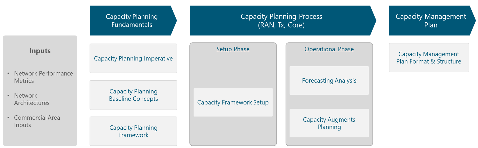
Figure 2 – CP Functional View

2 CP Fundamentals

This section provides an overview of the baseline concepts of the CP process and its relevance for NaaS operators. Furthermore, an examination of each of the CP process’ steps is provided to guide NaaS operators through their implementation.

2.1 CP Imperative

CP is the process of planning a network based on utilization, bandwidth, and other network capacity constraints. Furthermore, it’s a type of management process that assists network administrators in planning for network infrastructure in line with current and future operations.

CP involves calculating the capacity required to support the expected network growth and finding ways of making that capacity available via the implementation of capacity augments. Furthermore, CP ensures that the network capacity is utilized in the most cost-effective and timely manner.

The relationship between CP and Performance Management relies on their specific scope. Performance Management focuses on optimizing the existing network elements to improve the performance. In contrast, CP determines the future network requirements using the current performance as a baseline.

The main issues addressed by the CP process are examined as follows.

Avoid Capacity Outages

• Save Capital Expenditure (CAPEX) and Operational Expenditure (OPEX) due to Emergency Procedures
• Increase Customer Satisfaction / Reduce Churn
• Avoid penalties due to network unavailability periods

Minimize Idle Capacity

• Improve Return of Investment (ROI) speed
• Save OPEX spent on idle capacity
• Get better prices by ordering capacity augmentation just-in-time.

Improve Operational Efficiency

• Optimize capacity augments
• Reduction on Inventory
• Avoid delays in new services deployment and customer integration

Figure 3 illustrates the CP concept for NaaS operators. It maintains a CP process for each of the network segments (i.e., RAN, Tx, core) as each of them has particular requirements; however, interrelationships among the different processes are present. Each of these processes is described in a separate section of this module.

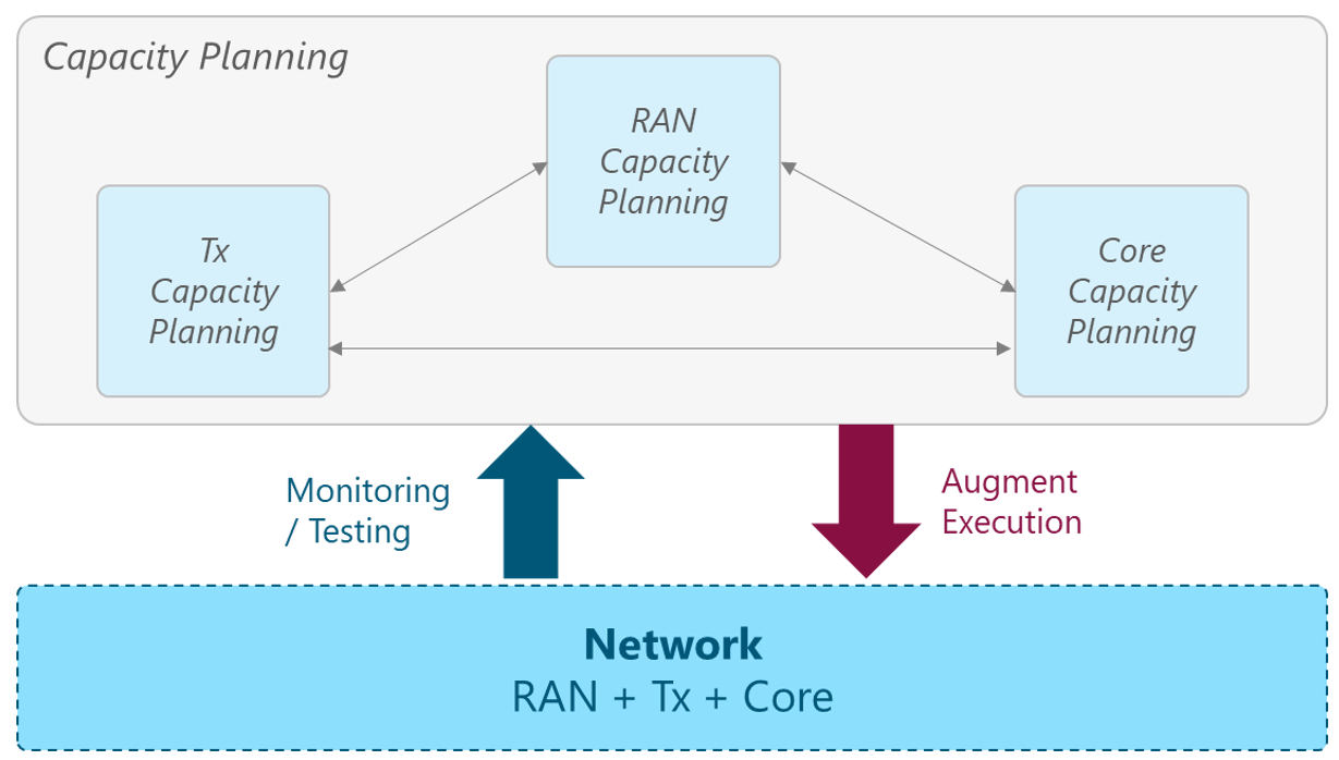
Figure 3 – CP Concept in the NaaS environment.

A deep examination of the fundamental aspects of CP can be found in the Primer on Capacity Planning Fundamentals document.

2.2 CP Baseline Concepts

The aim of this section is to present the key concepts related to CP that will be used along the rest of this module.

CMO

A CMO is a network resource that is capacity sensitive and is prone to present capacity outages. The CP process keeps track of three essential measurements for each CMO:

• Total Capacity All CMOs have some limit on their capacity, above which a degradation in their performance occurs. For instance, each base station has a maximum number of simultaneous subscribers that can be supported; in this way, the base station cannot support any additional subscriber when this number is surpassed. Another example can be the number of interface cards in equipment, which sets the total capacity of available physical interfaces on the network equipment.
• Utilization Utilization refers to the usage of the CMO over a determined period. In some elements, this might be very simple to count, for instance, the number of physical interfaces in use on a specific network element. However, for certain CMOs, the actual utilization may change rapidly (e.g., the amount of data transferred over a link). It’s important to note that utilization measurements can be performed using the associated network metrics. These network metrics are constantly monitored by the network monitoring system (NMS).
• Available Capacity The final vital element is derived from the first two, but it’s the most important to capacity managers. The available capacity indicates the amount of capacity that can be used in a CMO. When the available capacity is null, it’s said that the capacity of the CMO is exhausted.

Capacity Augment

A capacity augment is an expansion on any of the CMOs that augments its total capacity. There are mainly two approaches to augment the CMOs:

• Horizontal Augment: In this type of augment, additional CMOs of the same group are added to increase the capacity. A group of CMOs are elements with similar characteristics that are essentially interchangeable with any other. Moreover, horizontal augments increase the availability and redundancy of the network. On the other hand, the cost of implementing an additional CMO can impact the NaaS operator business case. An example of this type of augment is to add an additional Tx equipment when required.
• Vertical Augment: Vertical Augments refer to the expansion implemented to augment the total capacity of a specific CMO. For instance, the capacity of a router can be augmented by adding additional boards.

Capacity Augment Cycle Time

The capacity augment cycle time is the total amount of time required to implement a specific capacity augment. Among the activities that might be performed to implement a capacity augment are:

• Augment Design: Includes the time to generate the Methods of Procedure (MOP) document to implement the capacity augment. In some cases, a complete high-level and low-level design must be performed.
• Equipment/Spare Parts Delivery Time: Considers the time to retrieve the Tx Equipment / Spare Part from the NaaS Warehouse. In some cases, a new Product Order (PO) must be issued according to the Procurement procedures if the required elements are not available in stock.
• Site Visit: Most of the time, a site visit must be scheduled to apply the augments or perform a Technical Site Survey (TSS) to validate the feasibility of an augment. This time includes the transportation of staff/materials to the site.
• Installation & Commissioning: The required time to install the Tx equipment / Spare parts and perform the commissioning activities. Additionally, the testing time might require an acceptance procedure of the augment.

2.3 CP Framework

As previously discussed, CP has a direct relationship with the NaaS operator network, including all the network segments (RAN, Tx, Core). Figure 4 illustrates the CP framework.

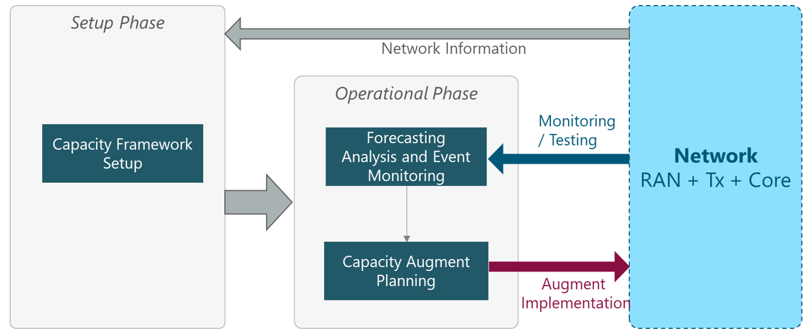
Figure 4 – CP framework

As shown in Figure 4, there are two phases in the CP process:

• Setup Phase: Defines the main elements (e.g., CMOs, capacity augments and cycle times) for the different network segments (i.e., RAN, Tx, mobile core). Furthermore, the network metrics to be monitored are defined for each CMO.
• Operational Phase: The objective of this phase is to adopt a structured approach to define the capacity augments required in the network to avoid network outages. To this end, the network utilization is monitored to determine future capacity requirements based on current and historical data.

The framework illustrated in Figure 4 is applied for each network segment (i.e., RAN, Tx, core). To facilitate understanding of the specifics, the rest of this section is focused on the generic approach, which will be used as the baseline for the specific processes on each network segment in Sections 3 to 5.

The following subsections describe the main interactions between the CP process and the NaaS Operator Network.

Initial Network Information Collection

The Capacity Framework Setup phase requires certain initial information regarding the network status. Table 1 presents the input data and their respective candidate sources. Furthermore, the impact of the inputs on the CP process is examined.

Table 1 – Initial Network Information Analysis

Monitoring / Testing

Monitoring and Testing activities focus on measuring and reporting all the utilization-related aspects. The NMS performs the capacity and performance monitoring activities. It’s recommended that automated mechanisms perform all monitoring activities.

The NMS utilizes inputs from the CP process to configure the Events & Alarms in accordance with safety margins for the network metrics. For further details on the monitoring techniques and how to implement them, please refer to the Network Monitoring Architecture module.

Capacity Augment Implementation

Once the capacity augments required in the network to avoid capacity outages are identified, they need to be implemented. Any capacity augment to be implemented in the network must be evaluated in terms of its impact on current service operation. Moreover, the implementation of the capacity augments must consider its associated cycle time to effectively schedule it.

The capacity augments follow a Capacity Management Plan, which details the activities to be performed for their implementation. This plan includes the sequence, relationships and time required to implement each of the capacity augments.

2.3.1 Capacity Framework Setup

The Capacity Framework Setup is the set of activities that defines the essential elements to execute the CP process based on the NaaS operator’s network characteristics. These activities include the definition of the network metrics to be monitored and their safety margins. Furthermore, they also include the definition of the options for capacity augmentation for each CMO and the estimation of their corresponding cycle times.

Figure 5 displays the elements that comprise the CP framework setup.

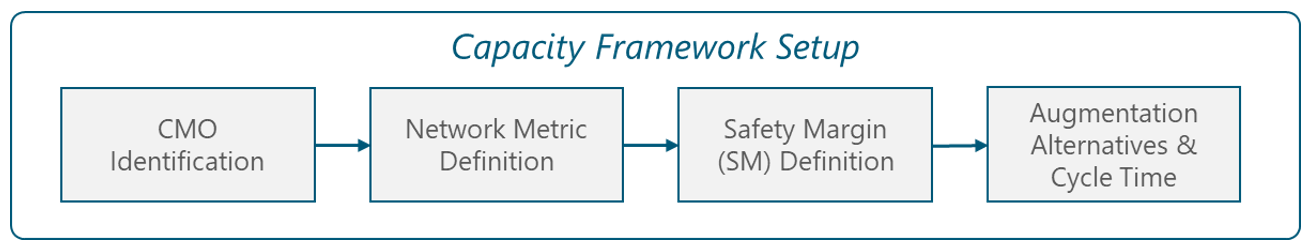
Figure 5 – Capacity Framework Setup

The following subsections examine the tasks performed as part of the Capacity Framework Setup.

2.3.1.1 CMO Identification

The first step in the Capacity Framework Setup is to identify the CMOs that will be considered in the CP process for each network segment (i.e., RAN, Tx, mobile core). To this end, a Top-Down approach can be followed to identify the CMOs in a structured approach.

The Top-Down approach starts analyzing the network elements at the device level, identifying the capacitive-sensitive elements prone to be exhausted. Then, for each of the identified devices, the analysis is repeated at the following level and so on. Figure 6 illustrates the Top-Down approach.

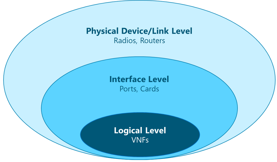
Figure 6 – Top-Down approach to identify CMOs

2.3.1.2 Network Metric Definition

Once the CMOs have been identified, a mapping to their associated network metrics must be performed. This step is important because the network metrics monitoring will determine the actual status of each CMO’s capacity.

The network metrics are measurable outputs that indicate the utilization of the network elements. There is a diverse array of network metrics available depending on the vendor and the network element technology. Careful selection of the most meaningful metrics to be monitored improves the accuracy of the CP process.

Each network metric can be associated with one or more CMOs. To identify the network metrics associated with a specific CMO, an examination of the available network metrics must be performed to determine which of them can be associated with a CMO.

2.3.1.3 Safety Margin Definition

A safety margin determines the maximum utilization supported by a network element when the performance is within the acceptable level. This safety margin is defined considering the average utilization of the network metric, to accommodate utilization peaks that may occur. When the network metric average utilization surpasses the safety margin, a degradation in the performance is presented.

In terms of capacity, a capacity augment must be implemented to avoid that the CMO’s average utilization reaches the defined Safety Margin and avoid potential capacity outages. Each CMO’s safety margins can be defined based on equipment technical specifications, industry standards or vendor recommendations.

2.3.1.4 Capacity Augments & Cycle Times Definition

Before passing to the operational phase of the CP process, the last step is to identify the alternative capacity augments for each CMO and their associated cycle time.

As stated in Section 2.2, there are mainly two approaches to augment the CMOs (i.e., Horizontal and Vertical). Each CMO must be examined to determine the possible augments to expand the capacity, depending on the specific technology and vendor.

Finally, to estimate the cycle time for a specific capacity augment, all the dependencies for their implementation must be considered. These activities might include the augment design, the equipment delivery time, the site visits and the installation & commissioning. In this way, the total cycle time is the sum of all the tasks involved in the implementation of the capacity augment.

2.3.2 Forecasting Analysis and Event Monitoring

Network Capacity Forecasting is a process to analyze the network growth over time. Subscribers’ growth implies a growth in the traffic carried by the network. For this reason, network growth is analyzed in terms of both the number of subscribers and traffic volume. As an essential part of the CP, capacity forecast aims to estimate future network behavior to predict when network utilization will reach network maximum capabilities and provide operators with proper time to apply network enhancements to overcome any issue due to capacity overload.

Capacity Forecasting provides NaaS operators the ability to predict future network behavior based on two factors:

• Network natural growth. The traffic in the network presents a natural growth due to several reasons (e.g., increment in the number of subscribers, percentage of active users in the busy hour (BH), average throughput per subscriber in the BH).
• Implementation of commercial strategies. These include different commercial strategies such as geographical network expansion, integration of new Mobile Network Operators (MNOs) into the NaaS infrastructure and new roaming agreements.

It must be noted that the forecasting analysis for the number of users is the only metric that will have a direct commercial growth component and a trending component as displayed in Figure 7. From this result, all the other network metrics will be estimated based on the forecasted number of users and the trending analysis.

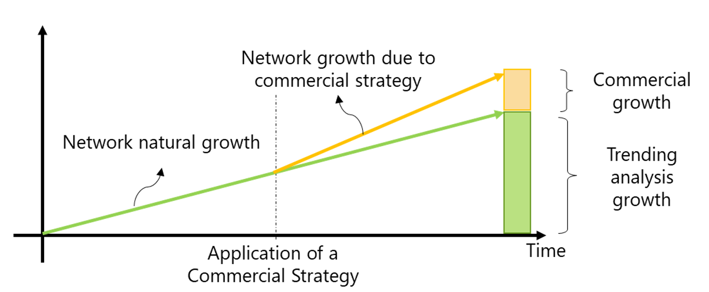
Figure 7 – Forecasting process composition of the number of subscribers.

Furthermore, forecasting analysis outcomes are used in later CP steps to develop successful preventive congestion control actions in the form of capacity augments to the network equipment and configurations. These augments target to avoid network congestion with respect to the forecasted traffic.

The ability to anticipate network congestion is critical for efficient service provisioning and intelligent decision making in the face of rapidly growing traffic, changing traffic patterns and aggressive market strategies. Proper network CP ensures that the NaaS operator is ready to overcome any capacity bottleneck in the network in an efficient way.

Figure 8 displays the forecasting analysis process for the network metrics that can be directly measured. As previously mentioned, it must be noted that some network metrics can be analyzed only by its trending behavior, without the influence of the commercial growth analysis.

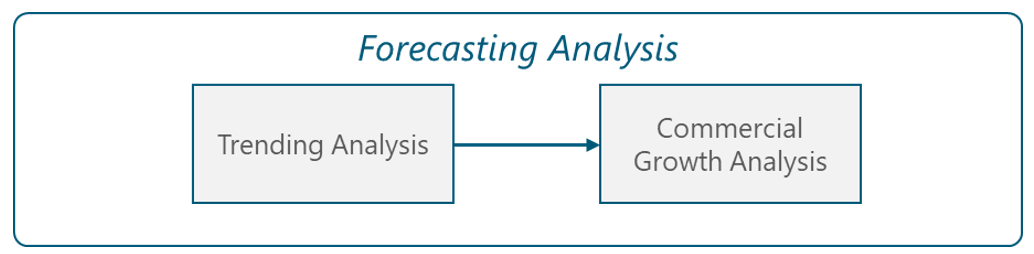
Figure 8 – Forecasting Analysis process.

The following subsections present the methodologies to estimate each of the above components using network monitoring data as the primary input.

2.3.2.1 Trending Analysis

Several methods for trending analysis have been studied in both academic and commercial fields. Among these methods, time-series data analysis represents a suitable technique in network traffic prediction in mobile networks.

The main concept behind time series forecasting is that the measure of some variable at a given time depends on the measure of the same variable at a previous time period, two time periods prior and so on. While no method dominates among others, a popular method that is usually applied in network forecasting is the Autoregressive Integrated Moving Average (ARIMA) model.

ARIMA is a time series model based on three main concepts:

• Auto Regression (AR): This means that the value of the forecasting variable depends on the past values of itself. This implies a correlation between past, present and future values.
• Integrated (I): For statistical reasons, ARIMA allows to predict future values by considering the difference between previous values instead of their actual ones.
• Moving Average (MA): This part works by analyzing how wrong previous predicted values were for the previous time-periods to make a better estimate for the current time period.

Figure 9 displays a graphical representation of time series prediction.

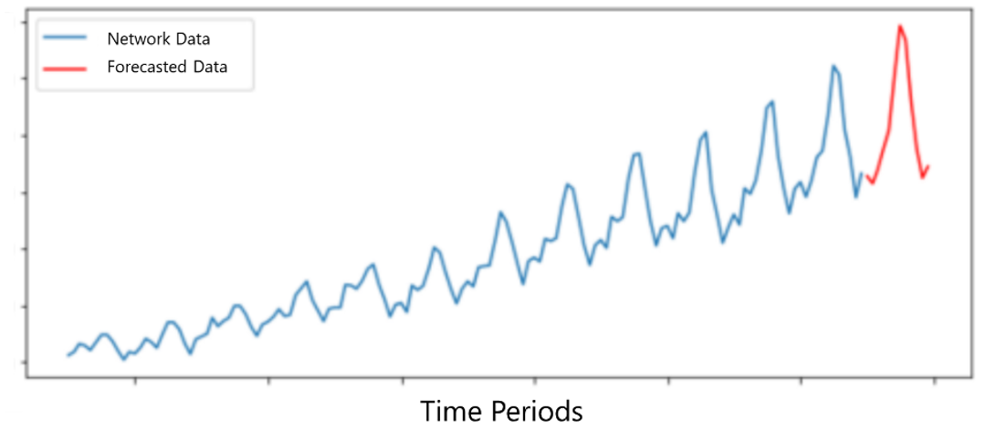
Figure 9 – Time series prediction using ARIMA method.

As it can be difficult and demanding to implement the ARIMA method, NaaS operators can utilize the Network Capacity Forecast Widget to generate the forecast of the network metrics using the ARIMA method presented in this section. Alternatively, NaaS operators may evaluate the purchasing of the XLSTAT tool for Excel which integrates ARIMA functionality. Deeper insight into forecasting analysis and methods will be addressed in the Network Capacity Forecast primer.

2.3.2.2 Commercial Growth Analysis

Commercial inputs can be provided in terms of the number of new subscribers or a growth percentage with respect to the number of existing subscribers. From this percentage, it’s possible to obtain the expected number of subscribers.

Once the final number of subscribers is obtained applying the commercial strategy, it can be used to forecast the rest of the network metrics that directly depend on it.

2.3.2.3 Event-Monitored metrics

There are certain metrics that can be directly obtained from monitoring systems and must be used to trigger the capacity augmentation based on utilization monitoring and event-based methods.

In this case, a capacity threshold should be established considering the provided guidelines. When the monitored metrics surpass the capacity threshold, a capacity augment should be implemented.

2.3.3 Capacity Augment Planning

The capacity augment planning provides the guideline to increase the capacity of a CMO before this is exhausted. The capacity augment planning process is illustrated in Figure 11.

The network metrics are collected and consolidated every time interval . Additionally, the CP process is performed every ‘periods. When a capacity augment is implemented, it takes ‘periods until the augmentation takes effect and the capacity is increased, which is the cycle time.

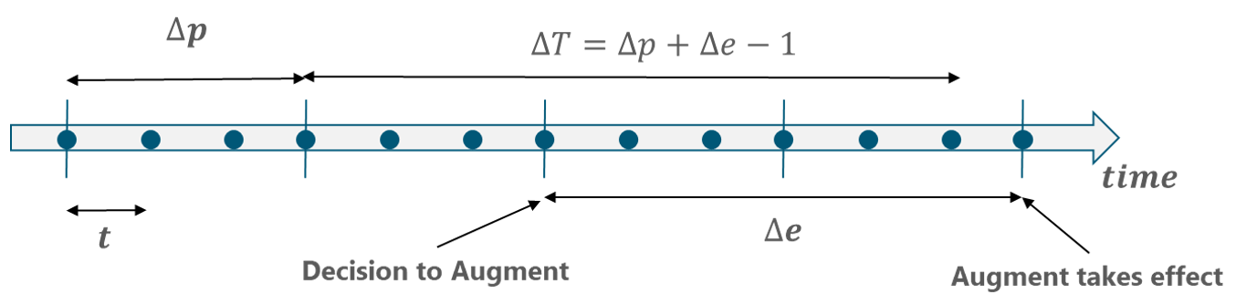
Figure 10 – Capacity augment Planning

As can be seen in Figure 10, some intervals should be defined to plan the capacity augments:

• Monitoring Period (t): According to the most common standards of the industry, the time for periodic monitoring is defined to be one week.
• Capacity Augment Cycle Time (): The factors that compose it are contained in section 2.3.3. Those components of cycle times may vary from one vendor to another and from country to country. When a CMO has more than one possible augment, it’s recommended to set this value to the longest cycle time. it’s usually measured in weeks.
• CP Evaluation Period (): This value is specific to the network segment in which the capacity process is implemented. This is because some network metrics are prone to vary abruptly in time, so they need to be analyzed more often. Therefore, the value of this time interval can fit into three categories according to its size: high, medium and low. Specific recommendations to define this value are provided in Sections 3 to 5 accordingly. It’s usually measured in weeks.
• CP Horizon (): The last piece for the forecasting formula is the minimum time horizon covered by the CP. From Figure 10, it can be calculated in the following manner:

(Eq. 1)

More details regarding the specific definition of these values are presented in Section 3 to 5, according to the network segment for which the CP process is performed.

To execute the capacity augments planning, certain activities must be performed. Figure 11 illustrates the activities related to the capacity augment planning.

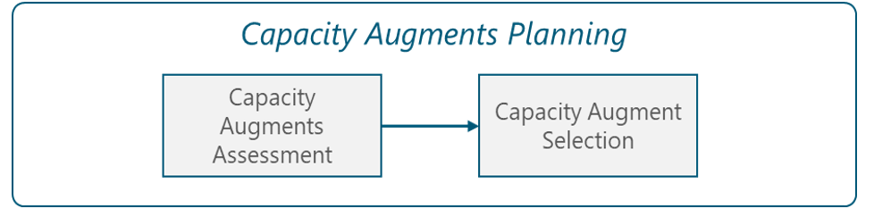
Figure 11 – Capacity augment planning process

2.3.3.1 Capacity Augments Assessment

To perform the selection of the most appropriate capacity augment, a score of the multiple alternatives must be performed to select the most appropriate for the NaaS operator. The most important components when deciding between options of a capacity augment are:

• Time. Is the total time required to implement the capacity augment (i.e., cycle Time). On special occasions (e.g., when the resource usage increases rapidly), time would be decisive due to the closeness of the action to take.
• Dependencies. A capacity augment may have dependency on others. In the case of such dependencies, the implications that a certain augment might involve must be clearly identified (e.g., a license application should always consider if the hardware would support it).
• Effectiveness. Reflects the increment in the capacity resulting from applying a specific augment. In certain cases, especially in mid-term horizons, it might be desirable to select an augment that provides a more significant increment in the capacity even though it might increase the cost.
• Cost. Cost might have a great impact on the selection. However, in some cases, an augment might not be the cheapest but the best cost-effective option.

The previous factors (with the exception of Dependencies) can be weighted through a ratio of importance (a, b & c), which can vary under certain circumstances. Eq. 2 to Eq. 5 illustrate how a specific capacity augment can be scored according to the parameters presented above.

	Eq. 2
	Eq. 3
	Eq. 4
	Eq. 5

Where:

• is the index for each capacity augment. The greatest means, the best suitable within the rank.
• are the ratios of importance for time, effectiveness and cost.
• is the cycle time of a certain augment () compared to the maximum cycle time of the set of augments considered (). Its values should be between zero and one.
• is the total capacity after a certain augment () compared to the minimum capacity of the set of augments ().
• is the cost associated with a certain augment () compared to the maximum cost of a set of augments (). Its values should be between zero and one.

Finally, the factors can be modified, varying the priority of the components according to different scenarios. Table 2 shows how these factors may vary to reflect the importance of the components in different scenarios.

Table 2 – Score factors for different scenarios.

2.3.3.2 Capacity Augment Selection

After the score for all the alternatives of capacity augments has been calculated, a selection of the most appropriate capacity augment can be performed by selecting the alternative with the highest score.

In Sections 3 to 5, specific examples regarding the different network segments (i.e., RAN, Tx and mobile core) are presented following the methodology described in the previous subsection.

Additionally, Naas operators can use the Capacity Augment Scoring Widget to perform the assessment and selection among multiple capacity augments.

2.3.4 CP Process Considerations

This section examines the required periodicity to execute the CP Process based on the network segment characteristics and the events that can impact CP by triggering an early analysis or pushing an urgent capacity augment.

2.3.4.1 Periodicity of CP Analysis

CP is a process that must be performed in a continuous fashion. The most common scenario to organize this process is to work on plans for multiple time horizons simultaneously.

For this reason, the CP process is performed in cycles based on the CP Evaluation Period for each network segment. In one cycle, the NaaS operator might finalize the plans for the next period and make provisional plans for the following period and outline plans for the period after that. Figure 12 illustrates the pattern in the cycles for the CP.

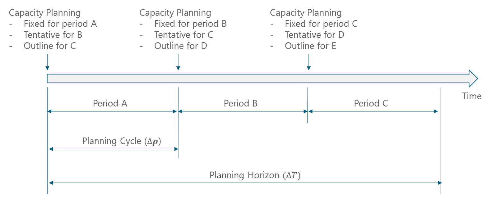
Figure 12 – CP Cycle Pattern

The pattern in Figure 12 facilitates the CP process because most operations are relatively stable, so the plans for one period can be used as the basis for the plans in the following periods.

2.3.4.2 Special Triggers for CP Analysis

Certain events are out of the control of the NaaS operator and have an impact on the network CMOs and their network metrics. These events can be seen as triggers for analysis of forecasting.

Commercial Inputs

Some commercial inputs can trigger an analysis because it impacts on the number of subscribers of the network. Some specific events are:

• Projection and implementation of new services
• Aggressive geographic expansion
• User consumption plan scheme modification
• Ceasing or New MNO/Roaming Agreements

Natural Disasters & Contingencies

This event is the most unexpected and has one of the most significant impacts on a country’s population’s daily life. Therefore, it impacts on the user’s mobility behavior and consumption.

Civil Infrastructure Modification

This event changes the mobility and consumption habits of the users. They even can make a specific area more or less concentrated in population. Some examples of buildings are:

• Supermarkets
• Stadiums
• Concert Halls
• Dense Residential Buildings

Special Events

The CP process should also consider certain events that will increase the number of users in some specific geographical areas and might cause the saturation on the mobile service (e.g., carnivals, processions, religious ceremonies).

⇐ Previous

3 CP in RAN

This section captures the specifics of the CP process applied to the RAN, including implications and dependencies for each step.

3.1 Capacity Framework Setup

In this section, the elements that comprise the Capacity Framework Setup for the RAN are defined following the procedures presented in Section 2.3.1.

3.1.1 CMOs

RAN resources can be divided into two layers: Carrier and Site level. The Carrier Level CMOs consider the available resources for users in the air interface while Site Level considers baseband processing and transmission resources of the eNodeB.

The RAN CMOs at the carrier level are listed as follows:

● Sector Carrier Resource Blocks: Physical resource blocks (PRBs) are the available resources at the carrier level. Increasing connected users or traffic volume leads to a continuous increase in the PRBs usage. As PRB usage approaches the maximum carrier capacity, user-perceived data rates will decrease.

● Connected Users per carrier: Each connected user consumes air interface resources. Therefore, as connected users increase, available carrier resources will become scarce and new users may fail to be admitted to the network.

The RAN CMOs at the site level are listed as follows:

● Connected Users per site: Every site has a certain number of configured connected user licenses. Each license allows a user to connect to the baseband unit (BBU) and consume both processing and transport resources. In addition, a site has a maximum user capacity that cannot be exceeded.

When the site reaches the maximum number of users connected with respect to its maximum configured licenses or with its user capacity, no more users will be admitted to the site, which means that the site cannot provide new services to new users.

● Downlink (DL) / Uplink (UL) Throughput: Just like connected user licenses, every site has throughput processing licenses to allow the BBU to process certain throughput volume. The amount of throughput licenses is limited by the maximum throughput that the BBU can process.

When user traffic reaches the number of throughput processing licenses configured at the BBU, the eNodeB performs flow control toward backhaul elements (i.e., BBU instructs cell site router to reduce the packet sending rate), affecting user experience in terms of data rate and service availability.

● BBU’s processing boards capacity: Each BBU is composed of a capacity processing board and a main processing board responsible for processing all data coming from the connected users. Capacity board processes user plane data while the main board processes control plane data.

When processing boards are close to reaching their maximum capacity, users may experience low constant access denial and constant connection drops. In the All-in-One (AiO) scenario, a BBU integrates both the capacity board and the main board into a single element, as described later in this section.

● Uplink port capacity load: The BBU has a limited number of Ethernet interfaces that serve as a physical interface toward the transport network. These interfaces carry user throughput and control plane traffic. When an interface reaches its maximum capacity, it loses its capabilities to transmit or receive data from the transport network, which is reflected in constant packet loss.

Furthermore, two scenarios can be defined for the RAN network equipment:

• Distributed Scenario: Where the radio unit (RU) is physically separated from the BBU.
• AiO Scenario: Where RU and BBU are integrated into the same box.

Even though both scenarios share the same CMOs, scenario separation impacts the capacity augments applicable to each one (as addressed in section 3.1.4.1) since an AiO site cannot handle the same capacity augments than a distributed site.

Carrier and Site level layers are applicable to the distributed site. However, for the AiO scenario CMOs are all considered at the site level since radio and baseband resources are shared.

3.1.2 Network Metrics

To perform the forecast analysis for CP, each CMO needs to be associated with a network metric. Thanks to this association, CP for each CMOs is addressed by forecasting its corresponding network metric. CMO’s network metrics are obtained from the NMS. RAN CMOs and their corresponding network metrics are shown in Table 3

Table 3 – RAN network metrics and CMO correspondence.

In addition to CMO related metrics, two additional metrics must be considered to impact the forecasting process:

Number of Subscribers (): This element is driven by the total number of users present on the NaaS Operator’s Network. ‘can be obtained as an input from the commercial team or can be directly measured from the current users in the live network.

Simultaneous Attached Users (): When a subscriber attempts and succeeds to connect to the Mobile Network, it’s then considered to be attached and ready to use network resources and establish communication. It’s important to note that the total number of attached users can be directly measured by network monitoring at different levels: at carrier level, at site level or at network level.

Busy Hour (BH): The number of simultaneous attached users varies depending on the hour of the day, consumption plans and population. The hour of the day with the greater quantity of simultaneous attached users is considered the BH; this is the period in which all metrics should be measured and forecasted. There is a possible scenario in which there is more than one BH of the day, in such cases and for simplicity, the hour with the greatest traffic and users should be considered.

The following subsections provide a description and definition for each RAN network metric shown in Table 3.

3.1.2.1 Sector Carrier Resource Blocks

PRB utilization must be measured for every carrier in the network. PRB utilization is given by the ratio between the PRBs in use () and the total amount of PRBs in the sector (). Eq. 6 displays this ratio.

Eq. 6

Both the used and are quantities that can be obtained directly from network monitoring. Moreover, is a constant value that only varies based on the carrier bandwidth.

3.1.2.2 Connected Users (per carrier & per site)

Connected Users CMOs are related to the . As mentioned before, can be considered at different levels depending on the metric to be analyzed. In this case, is considered at carrier level and at site level. Interactions between radio resource control (RRC) Connected User metrics and are as follows:

● User Utilization is the ratio between the at BH and the maximum number of supported users per carrier (). Eq. 7 displays this relation:

Eq. 7

● User License Utilization is the ratio between the at BH and the total number of user licenses configured at the BBU (). Eq. 8 displays this relation:

Eq. 8

3.1.2.3 BH Average User UL/DL Throughput

RAN monitoring systems allow to collect the total amount of DL and UL throughput carried by the eNodeB during the BH (). To obtain the throughput per user at the BH, must be divided by as follows:

Eq. 9

Eq. 10

Where:

● is the BH average user DL throughput.

● is the DL throughput carried by the eNodeB at the BH.

● is the BH average user UL throughput.

● is the UL throughput carried by the eNodeB at the BH.

Throughput Metric Considerations

It must be noted that some Network Management Systems might only be capable of reporting volume-related metrics in the form of data usage per subscriber at the BH. Therefore, a conversion function on the volume metrics must be performed to derive the throughput metrics in this case.

Considering that there can be multiple BHs during a day (typically =6 to 8), the formula to calculate the downlink throughput () from the monthly data received per subscriber () is in Eq. 11:

Eq. 11

Similarly, the UL throughput () can be calculated from the monthly data sent per subscriber ( ) as in Eq. 12:

Eq. 12

As an example, the throughput can be estimated for a subscriber with a monthly data usage of 1000 MB by considering 6 BHs in a day and using Eq. 11:

3.1.2.4 BBU’s processing boards capacity

Processing board utilization is a percentage that can be directly pulled out from the NMS via the corresponding network counter for both the processing unit and for the main unit.

3.1.2.5 Ethernet port capacity load

Ethernet transmission port utilization is a ration between the average Ethernet port rate () and the maximum rate supported by the port (). This relation is shown in Eq. 13:

Eq. 13

Where can be obtained during network monitoring and is a constant value for each BBU model.

3.1.3 Safety Margins

It’s worth mentioning that each equipment vendor can define its own safety margins to guarantee and optimal performance for its equipment. NaaS operators must look into the vendor’s documentation to ensure the vendor hasn’t already considered any different safety margins.

Table 4 displays the recommended safety margins (thresholds) for each utilization metric corresponding to each CMO. Threshold values for each network metric have been selected based on industry and rural network standards.

Table 4 – RAN network metrics safety margins.

3.1.4 Capacity Augments & Cycle Times

This section discusses available capacity augments for RAN considering the two scenarios options discussed in section 3.1.1: Distributed and AiO. Finally, a high-level approximation to the estimated implementation time of each of the augment is provided including the factors that impact such time.

3.1.4.1 Capacity Augments

Table 5 displays the recommended capacity augments to overcome capacity congestion on RAN CMOs. Notice that not every capacity augment can be applied to an AiO site.

Table 5 – RAN capacity augments.

3.1.4.2 Cycle Times

Each capacity augment involves various activities to carry them out. Duration for the implementation (cycle time) of each capacity augment depends on the activities involved in it and how NaaS Operator implements its site maintenance and logistics.

Table 6 displays general activities required for the implementation of each RAN capacity augment and an approximation to a high-level cycle time impact required for each one.

Table 6 – RAN capacity augments activities.

3.2 Forecasting Analysis and Event Monitoring

As discussed in section 2.3.2, the forecasting process plays an important role in the CP process to support future network growth. Through forecasting analysis, final capacity values are obtained, and capacity augments can be applied based on such outcomes.

Section 3.1.2 addressed the network metrics and the parameters related to them that are subjected to the analysis. This section guides the operator into the forecasting process of the RAN metrics applying forecast methodology shown in section 2.3.2.

Obtaining the final capacity values is a process that involves, in general terms, the following augments:

• Information on the current state (value) of the network metrics that impact each network metric.
• Historical network data of the forecasting quantities collected over a certain period: months, weeks, days.
• Commercial Inputs from strategy and commercial teams, which are composed of the expected number of new users.

Figure 13 summarizes the forecasting process that can be applied to RAN, transport and core networks.

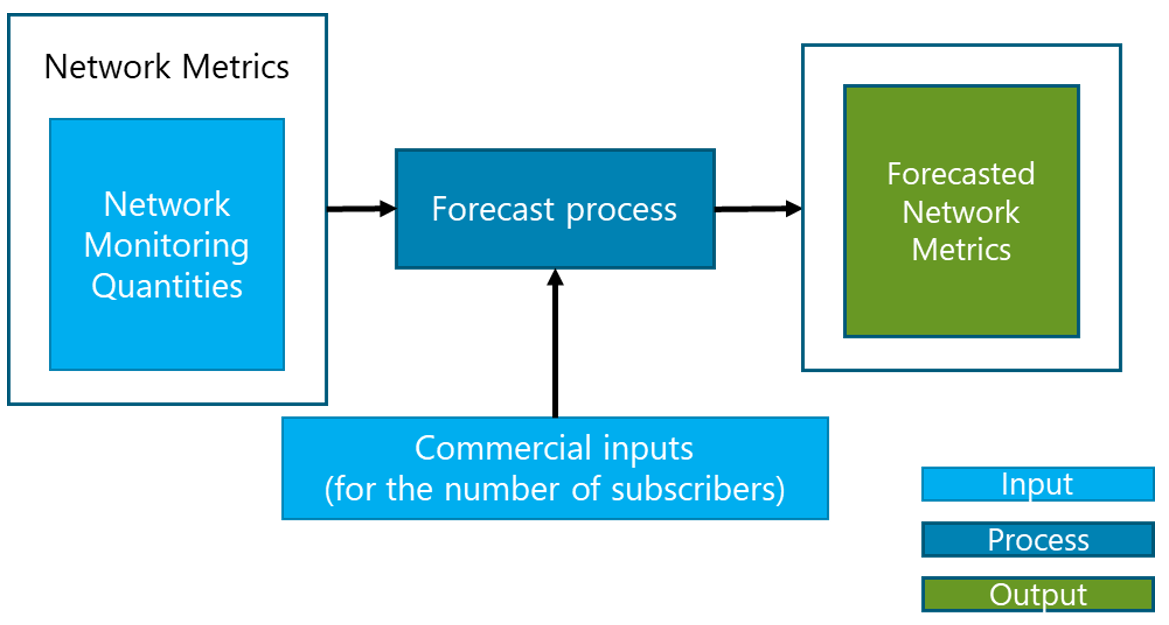
Figure 13 – Forecasting Process.

Table 7 summarizes which network metrics must be forecasted to compute the required network metric required in the CP process.

Table 7 – RAN network metrics forecasting summary.

It’s important to mention that all the forecast methods applied to the metrics in subsequent sections are based on the ones contained in section 2.3.2.

3.2.1 Forecasting

is a quantity whose forecast impacts several metrics, as seen in section 3.1.2. is a quantity that can be obtained from network monitoring, while is an input provided by the commercial team. The percentage of with respect to the is given by Eq. 14.

Eq. 14

Where:

is the percentage of SAU in the BH with respect to the total amount of subscribers in the region

To obtain the forecasted value of the , forecast analysis must be obtained for both the number of subscribers () and . This analysis should be performed with methods from section 2.3.2. Forecasted is obtained by adding the number of additional subscribers due to marketing plans with subscriber trends. On the other hand, is forecasted to obtain its forecasted value.

The forecasting process for is displayed in Figure 14.

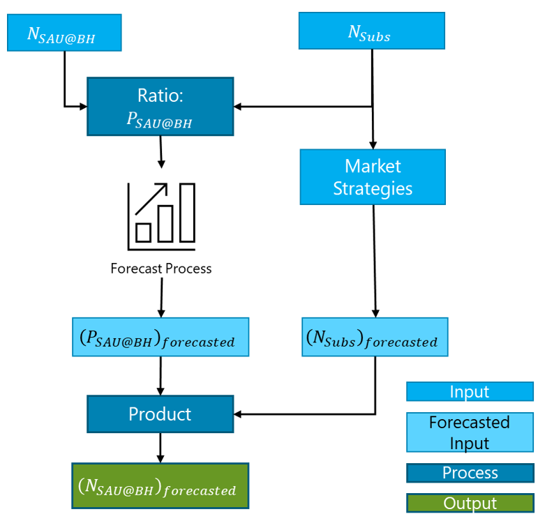
Figure 14 – Forecasting process for .

Eq. 15 summarizes the calculation of

Eq. 15

Where:

– is the forecasted number of subscribers in the region based on natural growth plus the additional ones added by commercial inputs. This commercial input must include the total number of subscribers considering all the MNOs utilizing the NaaS network.

Once has been computed, forecasting of the following network metrics can be directly obtained.

3.2.2 User Utilization and User License Utilization

and (Eq. 7 and Eq. 8, respectively) are constant quantities. Thus, forecasted User and User License utilization metrics can be obtained by forecasting the with the methods of section 2.3.2.1, at the corresponding level (carrier or site level) as shown in equations Eq. 16 and Eq. 17.

Eq. 16

Eq. 17

● For User Utilization:

o must be forecasted at the carrier level to obtain .

o The maximum number of supported users per carrier () is a constant value for each sector carrier.

● For User License Utilization:

o must be forecasted at site level to obtain .

o The total number of user licenses configured at BBU () is a constant value for each site.

3.2.3 DL / UL Throughput License Utilization

Resultant BH average user DL and UL throughputs (obtained from Eq. 9 and Eq. 10) must be forecasted and multiplied by the forecasted to obtain the forecast of the throughput per site as shown in equations Eq. 18 and Eq. 19:

Eq. 18

Eq. 19

● DL / UL Throughput License Utilization:

o must be measured and forecasted at the site level to obtain .

o and must be obtained as in Eq. 9 and Eq. 10 respectively using current network measurement values. Both quantities must then be forecasted using methods shown in section 2.3.2.1

o Figure 15 displays a graphical representation for obtaining the metric. The same applies to the UL throughput metric.

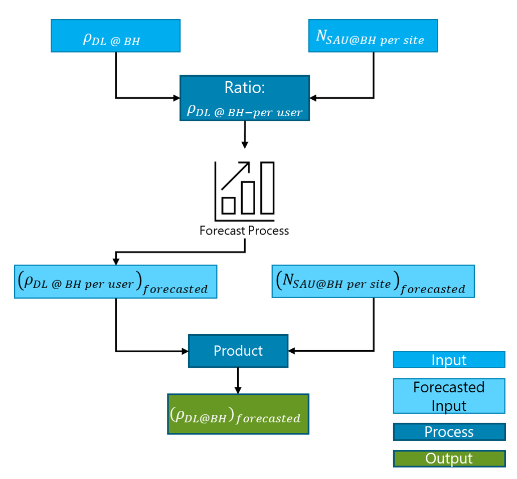
Figure 15 – DL Throughput License Utilization forecasting process.

3.2.4 Event-monitored Metrics

The following metrics can be directly obtained from monitoring systems and must be used to trigger the capacity augmentation based on utilization monitoring and event-based methods.

• PRB Utilization [%]
• Processing boards utilization [%]
• Transmission port utilization [%]

3.3 Capacity Augments Planning

As mentioned in section 2.3.3, since the implementation of each capacity augment requires certain time for its effects to be reflected as an enchantment of the CMO capacity, it’s necessary to determine when the analysis should be started to prevent capacity overloading and having enough time to implement a capacity augment.

On the other hand, some CMOs can be optimized by more than one capacity augment. In these situations, a NaaS operator needs to evaluate which one to implement.

To present an example that follows the methodology presented in section 2.3.3.1, Table 8 shows the required inputs to calculate the scoring values for each RAN capacity augment.

Capacity Augment	Cycle Time ()	Capacity after the augment ()	Cost () (for illustration Purpose only)
New Carrier	1 week	2k [users]	5k USD
New Sector	3 weeks	4k [users]	20k USD
New Site	16 weeks	2k [users]	Macro Cell: 60k USD
			Small Cell: 20k USD
Addition of new licenses	2 weeks	1.5k [users]1	5k USD
Update / Add Processing board	2 weeks	2k [users]	10k USD
Enable additional backhaul transmission port	2 weeks	2k [users]	2k USD
1 ‘ Will depend on the number of added licenses compared to the number of existing ones. Values in this table are assumptions and must be verified by the deployment team and vendor.

Table 8 – Scoring values for RAN capacity augments.

For example, considering a situation in which RRC Connected Users per carrier CMO is forecasted to be congested soon for a macro scenario. NaaS operators may choose between configuring a new carrier or deploying a new sector. The original capacity for RRC Connected Users is 1k users ().

From section 2.3.3.1, the score formula for capacity augments is equation 2:

For configuring a new carrier, score values will be as follows. For cycle time:

The Effectiveness is given by:

And finally, for cost:

Assuming the insertion of a new service scenario, the score of the capacity augment can be calculated as follows:

For deploying a new sector, the score is as follows:

It’s easy to see that configuring a new carrier is, by far, the best option in this situation. However, it has a dependency on ensuring that the installed equipment supports its addition. Moreover, the NaaS operator must review the impact in terms of coverage and network planning that this augment must make to the network.

3.4 CP Process Considerations

To know how often NaaS operators must carry out CMOs forecasting studies, it’s necessary to consider that some CMOs tend to change quicker than others. However, it’s impractical to compute different evaluation periods based on each CMO. The best approach is to compute a single evaluation period capable of involving all RAN CMOs into a single time frame. This can be done by analyzing the worst-case present in the RAN. In other words, the capacity augment that requires the time to be implemented.

For instance, the worst-case can be the New Site deployment augment. It can be assumed that this augment is triggered by the necessity of adding an additional BBU processing board. Thus, considering concepts introduced in section 2.3.3, one single augment horizon () can be obtained for RAN.

Table 9 shows a relationship between RAN CMOs and proposed values for .

Table 9 – values for every RAN CMO.

Based on these assumptions, computation of a single for the RAN based on the deployment of a new site can be done considering the following values:

● 12 weeks (corresponding to the BBU’s processing boards capacity CMO).

● 6 weeks (corresponding to the New Site cycle time).

Considering the methodology presented in Section 2.3.3, the augment horizon is computed as follows:

Thus, the forecasting process should at least cover the expected behavior of this CMO for at least 17 weeks. Finally, it must be considered that each capacity augment cycle time depends on how NaaS operator policies for the implementation of each capacity augment.

4 CP in Transport Network

The aim of this section is to examine the CP process applied to the Transport Network, its implications and dependencies for each step.

4.1 Capacity Framework Setup

In this section, the elements that comprise the Capacity Framework Setup for the Transport Network are defined following the procedures presented in Section 2.3.1.

4.1.1 CMOs

In the Transport Network, the CMOs can be divided into two categories.

The first category comprises the CMOS related to the Tx Link, responsible for transporting all the aggregated traffic among the base stations and the mobile core. The Tx CMOs on this category are as follows:

• Tx Link Utilization: The utilization over a specific Tx link is defined as the amount of traffic traversing it over a specific period of time. The Tx link can be implemented using different technologies (e.g., Fiber optic (FO), Microwave (MW), Satellite (SAT)). The Tx link utilization depends on the number of subscribers and the traffic generated by them.
• FO Utilization: Although the capacity over a FO is theoretically boundless (i.e., more than 30Tbps), the utilization of a FO link in NaaS operators is practically limited by the interfaces implemented on each side. However, an additional FO link can be implemented using an alternative FO strand over the same FO laying.

On the other hand, the other CMO category is related to the Tx Equipment, which are the devices that processes and forwards all the user and control traffic. The Tx CMOs on this category are as follows:

• Tx Interface Utilization: The main purpose of a Tx Interface is to enable communication among the devices in the transport network. However, when an interface reaches its maximum capacity, a degradation in its capabilities to transmit or receive data is presented, which is reflected in constant packet loss.
• Tx Interface Number: Each device in the transport network has a limited number of Tx interfaces. In some specific elements (e.g., router, switches), the number of interfaces can be augmented by installing an additional networking card.
• Tx Equipment Utilization: Each Tx equipment has a maximum processing capability to forward the traffic in the network. In this case, the Tx equipment utilization is directly related to the amount of traffic that needs to be processed.

The main purpose of a Tx Interface is to enable communication among the devices in the transport network. However, when an interface reaches its maximum capacity, a degradation in its capabilities to transmit or receive data is presented, which is reflected in constant packet loss.

4.1.2 Network Metrics

To monitor the actual status of each CMO, a mapping to their associated network metrics must be performed. Table 10 presents the network metrics associated with the Tx CMOs that need to be monitored by the NMS.

CMO	Network Metric [Units]	Periodicity
Tx Link Capacity	Tx Link Utilization [%]	15 min interval KPIs
Number of FO Strands	Available FO Strands [# of available FO Strands]	Monthly base
Tx Interface Capacity	Tx Interface Utilization [%]	15 min interval KPIs
Number of Tx Interfaces	Available Tx Interface Number [# of available Tx Interfaces]	Monthly base
Tx Equipment Capacity	Tx Equipment CPU Utilization [%]	15 min interval KPIs

Table 10 – Tx network metrics and CMO correspondence.

In addition to the mapping presented in Table 10, the following subsections provide a description and definition for each Tx network metric.

4.1.2.1 Tx Link Utilization

The Tx Link Utilization can be estimated by collecting the average throughput on the Tx link during the BH (). Then, the ratio between the average throughput on the Tx link and the total supported by the link can be calculated. This relation is shown in Eq. 20.

Eq. 20

Where:

is the total capacity of the link.

The link throughput can be calculated for UL and DL through Eq. 21.

Eq. 21

Where:

is the average throughput per user at the BH.

is the total number of sites that are aggregated in the Tx link. This number can be estimated by analyzing the network topology.

4.1.2.2 Available FO Strands

The number of available FO strands can be collected from the Network Inventory System and is strongly correlated to the Tx Link Utilization in FO links. If the latter reaches the safety margin in a particular FO link, an additional link can be implemented using an alternative FO strand, which will reduce the number of available FO strands by one every time it happens.

4.1.2.3 Tx Interface Utilization

At the interface level, the utilization can be estimated by collecting the average throughput on the Tx interface during the BH (). Then, the ratio between the average throughput and the total capacity supported by the interface can be calculated. This relation is shown in Eq. 22.

Eq. 22

Where:

is the average throughput in the Tx interface at the BH.

is the total capacity of the interface.

4.1.2.4 Available Tx Interfaces

The number of available interfaces can be collected from the Network Inventory System and is strongly correlated to the Tx Interface Utilization. If the latter reaches the safety margin (approximately 80% of the total capacity) in a particular interface, an additional interface needs to be used. Then, the number of available interfaces will reduce its number by one every time it happens.

4.1.2.5 Tx Equipment CPU Utilization

The Tx Equipment CPU Utilization is a Key Performance Indicator (KPI) that is commonly provided by the Network Performance System in percentage form.

4.1.3 Safety Margins

The compendium of safety margins for each of the Tx network metrics is represented in Table 11. Safety margins for the network metric have been selected based on industry and rural networks standards. However, it must be considered to consult the vendor’s own Safety Margins recommendations to guarantee and optimal performance for its equipment.

Network Metric	Safety Margin	Time Period
Tx Link Utilization	90%	Average percentages, 15 min interval KPIs @ BH
Available FO Strands	N/A	Assuming the capacity is examined each month.
Tx Interface Utilization	80%	15 min interval KPIs @ BH (BH)
Available Interface Number	2 Available for Aggregation Sites (Last-mile can stand 0 (zreo) available interfaces)	Assuming the capacity is examined each month.
Tx Equipment Utilization	80%	Average percentage @ BH

Table 11 – Tx network metrics Safety Margins

4.1.4 Capacity Augments & Cycle Times

Table 12 displays the recommended capacity augments to be considered in the Tx network.

Table 12 – Tx capacity augments.

Each capacity augment involves various activities to carry them out. The duration for the implementation of each capacity augment is known as the augment cycle time. It depends on the activities involved in it and how the NaaS operator implements them. Table 13 displays general activities required for the implementation of each transport capacity augment and an approximation to a high-level cycle time impact required for each one.

Table 13 – Cycle Time for Tx capacity augment.

It’s important to note that the NaaS operator should be able to correctly define the cycle times for every component. A complete survey with all the involved vendors and system integrators working with the NaaS operator can be helpful in gathering these times resulting in more accurate CP.

4.2 Forecasting Analysis and Event Monitoring

This section presents procedures to generate the Transport Network Capacity Forecast based on the identified network metrics and the inputs from the commercial area.

4.2.1 Tx Link Utilization

To forecast the Tx Link Utilization, the throughput per user can be forecasted using the methodology presented in Section 2.3.2.

Then, the total throughput in the Tx link for UL or DL can be forecasted through Eq. 23, by aggregating the traffic of all the sites aggregated over the Tx link.

4.2.2 Tx Interface Utilization

The Tx Interface Utilization can be forecasted by using the throughput per-interface since the interface capacity can be considered constant during the evaluation period. Eq. 24 displays the calculation to forecast the Tx Interface Utilization.

4.2.3 Available Tx Interfaces

Analogous to the available FO strands, the forecasting analysis of the available Tx interfaces is a challenge. Consequently, the forecasting for the available Tx interfaces is directly done by using the historical data from the NMS and applying the methodology presented in section 2.3.2.

4.2.4 Event-monitored Metrics

The following metric can be directly obtained from monitoring systems and must be used to trigger the capacity augmentation based on utilization monitoring and event-based methods.

• Tx Equipment CPU Utilization [%]
• Available FO Strands

4.3 Capacity Augments Planning

As discussed in previous sections, when there exist multiple capacity augments alternatives, the selection of the most appropriate is done through a scoring process applying the methodology presented in Section 2.3.3.

An augment in the capacity of a FO link whose original capacity is 1 Gbps () is taken as an example in the Tx Network. Table 14 displays three possible capacity augments that can be implemented. In this example, the capacity analysis is performed under normal circumstances.

Table 14 – Characteristics of capacity augments for fiber optic link.

It’s clear that are 8 weeks and 7.5k USD respectively. Since it’s a normal scenario, it’s advisable to select as 1, 1 & 1 respectively.

For option one, upgrade the interface capacity:

For option two, implement an additional link in alternative FO strand:

For option three, implement Additional Link in alternative FO path:

Therefore, the most appropriate augment in this specific case is to augment the interface capacity, which is the best scored alternative. The next augment according to their scores is to implement an additional link by using an additional fiber optic strand.

4.4 CP Process Considerations

Table 15 displays a summary of the CMOs and the recommended periodic times () for applying forecasting analysis and CP.

CMO	Recommended
Tx Link Utilization	Low
Available FO Strands	Medium
Tx Interface Utilization	Low
Available Interface Number	Medium
Tx Equipment Utilization	Medium
Low: 1’3 [week] Medium: 4’8 [week]

Table 15 – Recommended periodicity of analysis for each CMO.

The calculation of the augment horizon for the Transport Network () should cover all the possible scenarios. Network the greatest summed value of should be the one that drives all the other analysis.

As an example, the following table expresses the CMOs, their corresponding analysis periodic times () and their respective longest cycle times ().

Table 16 – Transport CMOs, and Examples.

Taking the methodology presented in Section 2.3.3, the result should be:

Therefore, the Augment horizon for the Transport Network during the CP process must consider at least the forecasting for 12 weeks ().

⇐ Previous

5 CP in Mobile Core

The aim of this section is to examine the CP process applied to the mobile core, its implications and dependencies for each step.

5.1 Capacity Framework Setup

As seen in previous sections, the identification of CMOs, their metrics, the safety margins for each metric and the subsequent capacity augments and cycle times is the previous work toward CP.

The following subsections will introduce and identify each of the components that will be used in the forecasting process.

5.1.1 CMOs

At the mobile core side, the CMOs slightly differ from the ones seen in previous sections. The main difference is that the Mobile Core Network is virtualized and the CMOs need to be subdivided into hardware and virtualized elements despite its inherent relationship. It becomes clear that those relationships will be translated into output/input between the elements of the Network Function Virtualization (NFV) solution.

According to the affinity of the element, the CMOs from the core side that are virtualized can be further subdivided into groups of Virtual Network Functions (VNFs). The mandatory subdivision is as follows:

● Control Plane (CP) VNFs (e.g., mobility management entity (MME), policy and charging rules function (PCRF)): Entities in charge of handling large amounts of signaling procedures from Simultaneous Attached Users.

● User Plane (UP) VNFs (e.g., serving gateway (SGW), packet data network gateway (PGW)): Elements whose main operation is to carry and process user data transmission. It’s driven by Simultaneous Attached Users & Traffic Profiles of each service present on the network.

● Database (DB) VNFs (e.g., home subscriber server (HSS)): VNFs in charge of storing all the user information from all the network. This group of VNFs requires large amounts of storage and processing for incoming and outgoing consults of the user registers.

On the other hand, the CMOs that correspond to the hardware infrastructure are the NFV infrastructure (NFVI) and the routing and switching equipment (e.g., switches and routers).

● R&S Equipment: Specific hardware whose principal tasks are to generate and process the routing and switching information, and to forward all the user-generated data toward its destination.

● NFV Infrastructure: Hardware responsible for hosting all the VNFs, the virtualization layer & the VNF manager. It can be composed of one or several physical servers working together.

5.1.2 Network Metrics

Different metrics are to be monitored for every CMO depending on the principal load they deal with. The following table shows the relationship between the CMOs and their main metrics.

Table 17 – Mobile Core CMOs and corresponding network metrics.

The metrics of each CMO have a tight relationship with each other and even with other CMOs. The relations are described in the following subsections.

5.1.2.1 CP VNFs

The Transactions per Second metric (TpS Load) is calculated considering the total amount of signaling procedures that the VNF will handle. Depending on the evolved packet core (EPC) element(s) that the VNF is representing, it will be the combination of signaling procedures. The following table summarizes the EPC elements on the control plane.

Table 18 – EPC Control Plane Entities and their corresponding signaling procedures.

Subsequently, the formula for calculating the Total Number of transactions per VNF at BH () will be:

Eq. 25

Where:

is the total number of Transactions at the BH.

corresponds to each of the types of Transactions that the VNF handles.

The signaling procedures are generated by the average Simultaneously Attached Users on the network at BH (). The quantity will vary according to their habits of mobility, session and usage of services. To calculate the transactions per second per user during the BH () corresponding to a CP VNF is by the relation of the total number of transactions that handles in the BH divided by the average number of users that are generating this signaling traffic (). The result must be converted to seconds (1 hour/3600 seconds).

Eq. 26

The metric of transactions per second per user must be calculated for different checkpoints along the network history as an input for the forecasting method. Then a method of forecasting should be applied to this metric.

If the result should be expressed as a percentage, the average number of TpS will be divided by the total capacity the VNF can handle and multiplying for a factor of one hundred. The following equation expresses the relation:

Eq. 27

Where:

is the TpS expressed in a percentage fashion.

is the capacity of TpS for a specific VNF.

It’s clear that since the is present in equations Eq. 26 and Eq. 27, as the SAU increases over time by different causes, the TpS Load will increase accordingly.

Finally, the CPU Load () is a metric that moves according to the average number of transactions per second. A ratio that relates both and can be considered as a constant is expressed as follows:

Eq. 28

Where:

is the ratio of processing load per transaction.

The is constant since the amount of processing resources per transaction does not change as the number of transactions or users increase. This relationship will later be used to estimate the amount of CPU Load for the forecasted users and transactions.

5.1.2.2 UP VNFs

For UP VNFs, the calculation is simpler since the most important metric will be the throughput and the active sessions/bearers that the users generate in the network.

For the throughput, it’s required to gather the KPI related to the total throughput (UL and DL) of the mobile network () and divided by the average number of users at the BH (). This throughput per user is expressed through Eq. 29.

Eq. 29

Where:

is the BH average user throughput.

A similar method should be applied to the active sessions. This is, the average number of active sessions per user at a given time, must be calculated as the result of the relation of the average number of active sessions during the BH divided by the average number of SAU. The previous analysis would result in the following equation:

Eq. 30

Where:

is the average number of active sessions per user at the BH.

is the average number of active sessions during the BH.

is the average number of SAU at a given time during the BH.

Later, the relationship of the average number of active sessions and throughput per user together with the forecasted values of users will drive the forecasted values of throughput and sessions that the mobile core infrastructure would handle.

5.1.2.3 DB VNFs

When it comes to DB VNFs, the imperative metrics are about the input/output operations for consulting the stored data and the number of users that conforms to the stored data.

There is a direct relationship for the Used Storage and the Subscriber Capacity Usage. The next formula shows the amount of storage needed per subscriber saved in the VNF.

Eq. 31

Where:

is the storage needed per subscriber.

is the total storage used to save subscriber information.

The final relation would be the Subscriber Capacity Usage that will result in Eq. 32:

Eq. 32

Where:

is the max number of stored subscribers supported by a DB VNF.

And the Used Storage metric will look much alike the Subscriber Capacity Usage. The following equation describes it:

Eq. 33

Where:

is the storage capacity of the VNF.

In the end, the relation of needed storage space for each user () will be used in combination with the forecasted subscribers to estimate the storage needed for the database VNFs.

5.1.2.4 R&S Equipment

The R&S equipment will rely entirely on the amount of traffic that the analyzed equipment is handling. The metrics will apply for every R&S entity along the network. The first metric in order is the Port Forwarding Load, which is driven by the port capacity. The relationship between these two is expressed in the following equation:

Eq. 34

Where:

is the average throughput of a specific port at BH.

is the port capacity.

The second metric is the available ports that can be gathered from the equipment inventory and is strongly correlated to the Port Forwarding Load. If the latter reaches the limit (approximately 80%) in a particular port, an additional port needs to be used and the available ports will reduce its number by one every time it happens.

Finally, the last metric is the CPU load of the equipment, which is a Key Performance Indicator (KPI) that is commonly provided by the Network Performance System in percentage form.

5.1.2.5 NFV Infrastructure

The hardware infrastructure is a result of all the above subsections and the relations are given by the virtualized resources that the VNFs and the R&S equipment demand.

For the CPU Load, the relation comes from the available vCPU, total vCPUs and the vCPU usage. The infrastructure should balance the processing load between the vCPUs supporting a certain VNF. Hence, if a VNF is demanding a certain number of processors because of its high usage, it will impact on the available vCPUs of the NFV infrastructure.

Eq. 35

This metric should not be directly forecasted since the used vCPUs are the result of the VNF demands to the NFV Infrastructure. This demand of vCPUs is the outcome of the forecasting analysis of each VNF metric for each VNF Type.

The same principle is applicable to the available storage and available RAM. The equations will end up as:

For Storage:

Eq. 36

For RAM:

Eq. 37

For Forwarding Capacity:

Eq. 38

5.1.3 Safety Margins

The compendium of metrics and the CMOs are represented in Table 19. It must be considered to consult the vendor’s own recommendations of Safety Margins before using the ones in the table. These recommendations are purely based on the premises that:

Higher Safety Margins: Metrics with high margins that do not affect the overall performance. These are limits that may be overcome with changes in software or minor changes in hardware such as TpS Load, Active Session Load, Total throughput, Subscriber capacity.

Lower Safety Margins: Metrics whose margins do affect the overall network performance. These metrics impact hugely when reaching critical limits due to its inherent properties. For example, the CPU Load since the CPU generates more heat than it dissipates hence degrades its performance closer to 100% load. Other examples are used storage, forwarding load and significant changes in hardware (NFVI and R&S Equipment).

Table 19 – Relationship between the Mobile Core CMOs and their safety margins.

When a certain metric is forecasted to reach these margins, it’s strongly recommended that an augment takes place according to the available options and the cycle times of the next subsection.

5.1.4 Capacity Augments & Cycle Times

The augments according to the metrics of each CMO are indicated in the Table 20.

Table 20 – Relationship between the Mobile Core Metrics and their possible capacity augments.

After the analysis for the augments according to the metrics of each CMO, it becomes clear that some of the capacity increasing actions are duplicated along the table. The unique augments are described in Table 21.

For the definition of cycle times, it will depend on the vendor response times, logistics and agreements with the NaaS operator. The cycle times will also be subject to the logistic, the available human and technical resources and the NaaS operator expertise. The following table encompasses the augments and their respective cycle times variables.

Table 21 – Relationship between the Mobile Core capacity augments and their corresponding cycle times.

The cycle times components shown in Table 21 must be summed up to obtain a total time for which the augment will take effect. This cycle times are also known as , as previously explained in section 2.3.3.

It’s important to note that the NaaS operator should be able to correctly define the times for every component. A complete survey with all the involved vendors and system integrators working with the NaaS operator can be helpful gathering these times resulting in more accurate CP.

5.2 Forecasting Analysis and Event Monitoring

The following subsections discuss the inputs and considerations related to the forecasting process regarding the metrics of section 5.1.2.

5.2.1 CP VNFs

From section 5.1.2.1, when the number of TpS per user at the BH increases, the CPU Load will rise accordingly and since the ratio of TpS per processing load is a constant it can be denoted as:

Eq. 39

The TpS Load would also increase accordingly to the total number of transactions per second in the network. The equation Eq. 40 represents this relation:

Eq. 40

In summary, the ratio and the metric that need to be forecasted are and .

5.2.2 UP VNFs

On the other hand, the BH average user throughput can be forecasted by any method of preference as seen in section 3.2. This throughput metric considers the UL plus the DL and, in contrast to the analog RAN metric, this average user throughput considers the traffic from the whole mobile network. Finally, the forecasted average user throughput is multiplied by the number of forecasted average simultaneous attached users at the BH to calculate the total amount of traffic data of the network at the BH.

Eq. 41

The same method should be applied to the active sessions since it has a tight relationship with the SAU. The previous analysis would result in the following equation:

Eq. 42

Where:

is the forecasted average number of sessions per attached user at the BH.

In summary, for the UP VNFs, the ratios and the metrics that must be forecasted are , and .

5.2.3 DB VNFs

From section 5.1.2.3, since the needed memory per subscriber won’t vary in time and can be considered a constant, so when the subscriber number augments, the required storage will do as well. The equation Eq. 43 shows the resulting calculation for the needed space.

Eq. 43

The final relation would be the Subscriber Capacity Usage that will result in the equation Eq. 44:

Eq. 44

And the Used Storage metric will look much alike the Subscriber Capacity Usage. The following equation describes it:

Eq. 45

In summary, for the DB VNFs, the only metric that need to be forecasted is .

5.2.4 R&S Equipment

The forecasting of the R&S equipment must be done considering two metrics: the available transmission ports and the equipment forwarding load.

For the port forwarding load, the throughput per port is the variable that increases over time and it has to be forecasted. Since the port capacity can be considered a constant unless upgraded, the equations from section 5.1.2.4 will result in:

Eq. 46

In summary, for the R&S Equipment, the metrics that need to be forecasted is ,which is purely a forecasting from the historical data and expected throughput from new sites or new services. is .

5.2.5 Event-monitored Metrics

The following metrics can be directly obtained from monitoring systems and must be used to reactively apply the capacity augmentation based on utilization monitoring and event-based methods:

• Used vCPU [vCPUs]
• Processing Load [%]
• Used Storage [%, GB]
• Used RAM [%, GB]
• Port Forwarding Load [%]
• Total throughput load [%]

5.2.6 Summary

From the previous section, the variables that are subject to a forecasting method from section 2.3.2 are contained in Table 22:

Table 22 – Compilation of forecasted variables for Mobile Core.

5.3 Capacity Augment Planning

As discussed in section 2.3.2, when there is more than one possible augment to the capacity of the network, the decision should be taken according to the current situation of the NaaS operator. The methodology to perform the scoring and selection of the most appropriate capacity augment is presented in section 2.3.3. It’s remarkable that all the augments in the Mobile Core network should follow the previous formula.

For example, three augments which are described in Table 23 can be applied for increasing the number transactions per second in the network. The current capacity of the system () is 100 [TpS]. The actual situation indicates that the NaaS operator is under normal circumstances:

Table 23 – Characteristics of capacity augments for number of active users’ metric.

It’s clear that are 3 weeks and 10k USD respectively. Since it’s a normal scenario, it’s advisable to select as 1, 1 & 1 respectively.

For assigning more vCPU to the CP VNF:

For adding more VNFs for the control plane:

For adding a new license:

Although for assigning more vCPU to the CP VNF has the dependency of checking if the hardware capacity allows it, this is the best option since it has the highest score. The next augment in order is adding a new license that has the same dependency as the first to the hardware.

5.4 CP Process Considerations

Table 24 displays a summary of the CMOs and the recommended periodic times for applying forecasting analysis and CP.

Table 24 – Recommended periodicity of analysis for each CMO.

When calculating an augment horizon () for the entire Mobile Core Network the greatest summed value of should be the one that drives all the other analysis.

As an example, the following table expresses the CMOs, their corresponding analysis periodic times () and their respective longest cycle times ().

Table 25 – Mobile Core CMOs, and .Examples

Taking the methodology presented in Section 2.3.3, the result should be:

The forecasting method should at least cover the expected behavior of all CMOs for 13 weeks ().

6 Capacity Management Plan

This section provides the methodology to consolidate and generate a final Capacity Management Plan, which is the main deliverable of the CP process.

6.1 Capacity Management Plan Format & Structure

The Capacity Management Plan contains the following aspects:

• Overview and Scope: High-level description of the scope of the capacity plan, including the network segments in examination, the involved stakeholders,

Furthermore, for each of the network segments (i.e., RAN, Tx and core), the following sections must be included:

• Network Metrics Performance Report: Historical report of the network metrics that monitored the behavior of the CMOs.
• Forecasting Analysis: Estimation of the network behavior according to the established time horizons for each of the network metrics and their associated CMOs. This section must highlight the possible capacity outages in each network segment that may occur if capacity augments are not applied.
• Capacity Augments Selection and Scheduling: Description of the plans for the capacity augments to be implemented and how they’ll be addressed and managed.

Finally, NaaS operators can use the $$link_widget$$Capacity Management Plan Template as a reference document to create their own version.